Stability of PC- and Varimax-rotations with different samplesizes.
In this discussion I want to find some rationale for the idea of "confidence interval" for the loadings of a pc- or a varimax/"little jiffy" or a PAF solution.
While I've dealt much experimentally with PCA and FA and rotations and although I know the basics about the Bartlett's sphericity test and the KMO-test I've not yet understood the idea of confidenceintervals for the loadings of a PCA or PAF solution.
Here I try to get some intuition about this by bootstrapping: doing PCA resp. PAF on random-samples from a given population which has a known correlation-matrix/factor structure.
The first idea was to have the nullhypothesis of zero-correlation in the population, but the statistics of the factor-loadings in, say 256 samples on N=40, was extremely variant and seemed to be useless for my goal of getting a primary intuition in a first overview.
Thus, for a first step into that difficult matter, I generated the following correlation-matrix from four items of synthetical data for the population, to have a certain stability in the pc-analyses of the samples at all. (link to data see end of article).
This is the correlation matrix in the population:
|
correlations |
item1 |
item2 |
item3 |
item4 |
|
item1 |
1 |
-0.632015 |
-0.676744 |
-0.367133 |
|
item2 |
-0.632015 |
1 |
0.131210 |
0.793069 |
|
item3 |
-0.676744 |
0.131210 |
1 |
-0.098988 |
|
item4 |
-0.367133 |
0.793069 |
-0.098988 |
1 |
Now I did four different common models of PCA and PAF for the population to see how the random sampling would reproduce the same structure if small or if medium sized samples are drawn.
First I assume that in the population there are true factors such that the items mark them correctly if they are in their pc-rotated position. I got the following pc-solution for the population:
|
PC loadings |
ax1 |
ax2 |
ax3 |
ax4 |
|
item1 |
0.869838 |
0.398677 |
0.202446 |
0.208455 |
|
item2 |
-0.897988 |
0.336709 |
-0.164272 |
0.230782 |
|
item3 |
-0.474966 |
-0.840259 |
0.235375 |
0.113891 |
|
item4 |
-0.738234 |
0.600784 |
0.286920 |
-0.108382 |
Next I assumed that in the population there are true factors such that the items mark them correctly if they are in their varimax-rotated position. I got the following varimax-solution for the population:
|
varimax loadings |
ax1 |
ax2 |
ax3 |
ax4 |
|
item1 |
0.163002 |
0.415617 |
0.835045 |
0.321548 |
|
item2 |
-0.446841 |
-0.037360 |
-0.331388 |
-0.830132 |
|
item3 |
0.087863 |
-0.929865 |
-0.356629 |
-0.021140 |
|
item4 |
-0.890561 |
0.088557 |
-0.147792 |
-0.420971 |
Third, I assumed that in the population there are true factors such that the items mark them correctly if they are in their "little jiffy" rotated position. The following is that composition of the items in the population:
|
varimax loadings |
ax1 |
ax2 |
ax3 |
ax4 |
|
item1 |
0.436552 |
0.851460 |
0.202446 |
0.208455 |
|
item2 |
-0.913752 |
-0.291224 |
-0.164272 |
0.230782 |
|
item3 |
0.146895 |
-0.953965 |
0.235375 |
0.113891 |
|
item4 |
-0.951684 |
0.015074 |
0.286920 |
-0.108382 |
Finally I've assumed that in the population are two paf-factors and residual variance and covariance. The residual variance is not diagonal, so I document here that (co)variance (in pc-rotated position of their loadings in ax3 to ax6)
|
paf (2) |
common |
loadings of residual covariance (in pc-position) |
|
|
ax1 |
ax2 |
ax3 |
ax4 |
ax5 |
ax6 |
|
item1 |
0.846 |
0.376 |
0.034 |
0.071 |
0.371 |
0.010 |
|
item2 |
-0.900 |
0.353 |
-0.013 |
-0.014 |
-0.012 |
0.256 |
|
item3 |
-0.458 |
-0.786 |
0.048 |
0.407 |
-0.067 |
0.008 |
|
item4 |
-0.678 |
0.531 |
0.506 |
-0.044 |
-0.019 |
0.005 |
* Normalization of signs of the components/factors:
The axes/components are in all samples were normalized such that the sign of the first component is positive in all axes.
In varimax and "little jiffy" it was also sometimes needed to exchange the first two axes to achieve best match with the population loadings. However still some samples are so distorted that the automatic procedure for this didn't detect the need for normalizing or did normalizing although not needed. I did not intervene manually
1) Confidence intervals for PC-loadings
I assume that in the population there are the true factors such that the items mark them correctly if they are in their pc-rotated position.
For bootstrapping I draw a set of S=256 random samples of sizes N=40 and in each sample found the empirial pc's as estimators for the PC's in the population. (That axes are normalized as in the population such that item 1 has positive loadings in all dimensions/axes)
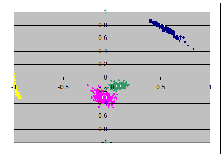
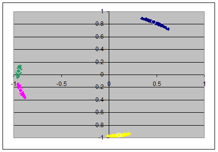
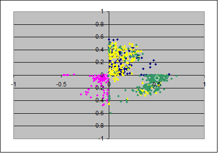
From the loadings-matrixes I produced scatterplots, each in two dimensions from pairs of axes. The pairs (x,y)-axes are: (ax1,ax2), (ax2,ax3), (ax3,ax4).
This gives the upper row of 3 scatterplots, and the colors indicate as follows: item 1 in blue, item 2 in magenta, item 3 in yellow and item 4 in green.
The loadings in the population's loadingsmatrix are marked with small white circles and are roughly in the mean of the colored clouds of points.
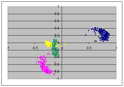
After that I draw another set of S=256 random samples, but now with each having N=160 observations. In the second row of the images below we see the scatterpots of that other empirical items's loadings.
PC
|
N=40 (x,y)=(ax1,ax2) |
(x,y)=(ax2,ax3) |
(x,y)=(ax3,ax4) |
|
|
|
|
|
N=160 (x,y)=(ax1,ax2) |
(x,y)=(ax2,ax3) |
(x,y)=(ax3,ax4) |
|
|
|
|
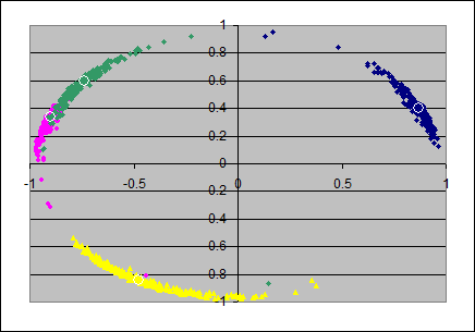

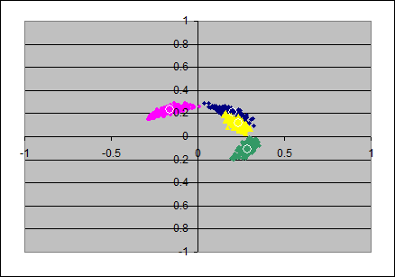
For the PC-solutions it seems, that the first and second principal components are much stable in their eigenvalues (the clouds seem to lay tightly on the circumference of some circle) but that the angular position of the items can vary considerably. (Which is surprising to me)
The stability of the eigenvalues in the lower principal components seem to decrease as well as the angular variation increases. Note that in the second and third scatterplot there are some green and magenta extremal points are visible in the two left quadrants; I think this is due to suboptimal normalizing of the axes: likely here it would have been appropriate to have the loadings of the first item negative.
Of course the impression improves if N=160 instead of N=40 is taken for the sample-size: we see that the variation around the populations' loadings reduces when the size of the sample increases.
Also the likely error by false normalizing of the loadings in the lower axes disappears now.
2) Confidence intervals for varimax-loadings
I assume that in the population there are true factors such that the items mark them correctly if they are in their varimax-rotated position.
For bootstrapping I draw in the same way as in section 1) S=256 random samples of sizes N=40 and in each sample found the empirial varimaxes as estimators for the varimax-loadings in the population. (The varimax rotation went over all four factors)
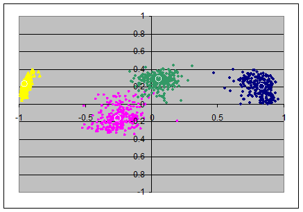
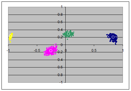
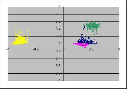
From the loadings-matrixes I produced scatterplots, each in two dimensions from pairs of axes in the loadingsmatrices. The pairs (x,y)-axes are: (ax1,ax2), (ax2,ax3), (ax3,ax4).
This gives the upper row of 3 scatterplots, the colors indicate again as follows: item 1 in blue, item 2 in magenta, item 3 in yellow and item 4 in green. The loadings in the population's loadingsmatrix are marked with small white circles and are roughly in the mean of the colored clouds of points.
After that I draw another S=256 random samples, but now with each having N=160 observations. In the second row of the scatterplots below we see the scatterpots of that other empirical items' loadings.
Varimax
|
N=40 (x,y)=(ax1,ax2) |
(x,y)=(ax2,ax3) |
(x,y)=(ax3,ax4) |
||
|
|
|
|
||
|
N=160 (x,y)=(ax1,ax2) |
(x,y)=(ax2,ax3) |
(x,y)=(ax3,ax4) |
||
|
|
|
|
||
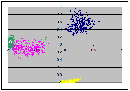

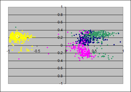
For the varimax-solutions we find less surprising plots: all "clouds" of the random samples appear as little "galaxies" of approximately circular shape: the radial as well as the angular deviations from the population's loadings seems to be random.
The amount of the deviations from the population's loadings in the varimax axes seems roughly constant over all pairs of axes.
However note that in the first and second scatterplot (N=40) there are some green and magenta extremal points are visible in the first quadrant; I think this is due to suboptimal normalizing of the axes: in a few number of samples the automatic normalization by the sign of the first item was not helpful.
Again (as in the PCA-examples) the impression improves if N=160 is taken for the sample-size. We see that the variation around the populations' loadings reduces when the size of the sample increases.
Also the likely error by false normalizing of the loadings in the lower axes does now no more occur.
3) Confidence intervals for the "little jiffy"
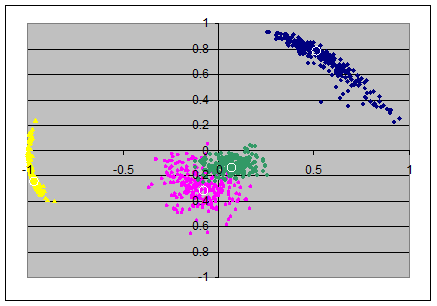
Here assume that in the population there are true factors such that the items mark them correctly if they are in their "little jiffy" position which means: principal components, then varimax-rotation in the first two axes (eigenvalues>1) only, but rescaled to have variance 1 on that two factors (which means "Kaiser-normalization" in SPSS).
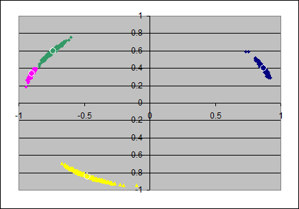
For the "little jiffy" with N=40 it was more difficult to find a rule for automatic normalizing the signs of the loadings - I even needed sometimes to exchange the first and the second axis to not to lose match with the population's "little jiffy".
Little Jiffy
|
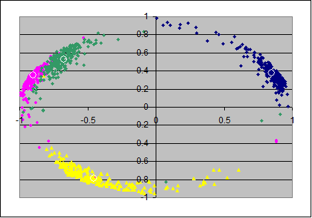
N=40(x,y)=(ax1,ax2) |
(x,y)=(ax2,ax3) |
(x,y)=(ax3,ax4) |
|
|
|
|
|
N=160 (x,y)=(ax1,ax2) |
(x,y)=(ax2,ax3) |
(x,y)=(ax3,ax4) |
|
|
|
|

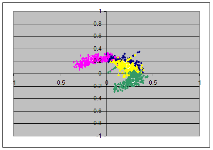

The elliptic/circumferential shape of the clouds in the two left scatterplots look as if there is a combination of the advantages of each of the two involved rotations combined: the radial distortion is as small as in the pc-model, and the angular distortion seems smaller than in the simple pc-model (but perhaps a bit wider than in the full varimax model). The third and fourth axes are not changed from that what they had after pc-rotation.
4) Confidence intervals for PAF (2 factors)
Here I bootstrap for the hypothese for the population that it has two (PAF-)factors, unique variances and a minor residual correlation.
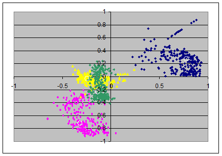
The two PAF-factors leave in general spuriously correlated errors, so the axes ax3,ax4 should be accompanied with ax5 and ax6 to cover the full space of residual (co)variance.
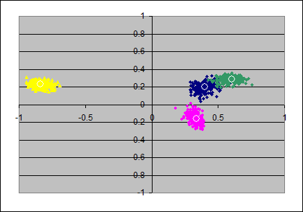
Although the residual variance/covariance follows a different logic than in PCA I've just added the first 2 principal components of the residual covariance matrix in the place of ax3 and ax4, so only the first and the third scatterplots in the rows below should be really informative.
PAF(2)
|
N=40 (x,y)=(ax1,ax2) |
(x,y)=(ax2,ax3) |
(x,y)=(ax3,ax4) |
|
|
|
|
|
N=160 (x,y)=(ax1,ax2) |
(x,y)=(ax2,ax3) |
(x,y)=(ax3,ax4) |
|
|
|
|
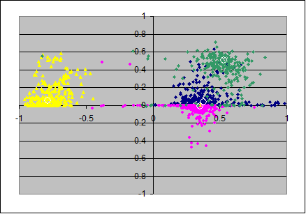


The two left scatterplots look as weaker estimates than that from the pc-model. Most of that impression might reflect the fact that the communality of the involved items varies with the samples (and also often jointly) stronger than in the pc-model.
Original data: To be able to reproduce the scatterplots you may use the rawdata at confidenceforloadings.csv
Little Jiffy: The term "Little Jiffy" was coined by the workgroup around H. Kaiser in the 1960ies as stated in H. Kaiser's article "Second generation Little Jiffy" in Psychometrika
Computation were done with MatMate (proprietary matrix calculator software), pictures created with MS-Excel
Gottfried Helms, Kassel, 15.7.2015