|
|

Tetration of a small base 0<b<e-e via regular
iteration
using the repelling fixpoint
A provisorical computation
for newsgroup-discussion
using Pari/GP
Version 1.2
Gottfried Helms, 28.06.2009
1. Provisorical computation of values for tetration with a base 0<b<e-e ; example b=0.04
The following is a very provisorical discussion of the regular iteration of tetration with an unusual base 0<b<e–e. There are some facts known and discussed, see for instance [1,2,3] in the "tetration-forum", but here I consider some specific matters using an example base.
The numerical approximations may be of much improvable quality (although I used matrix-size of 64x64 which usually gives at least 10 digits of accuracy), but is not of too much concern: the article may serve as a general impression of basic behaviour when such bases are involved in tetration.
1.1. Function-graphs of integer iterates of bx
First, let us see a graph for some integer iterates of Tb°h(x); here we look at heights h=0 (the linear function f(x) = x) , at h=1 , the base-function Tb(x) = bx, then at h=2 where Tb°2(x) = bbx , then at h=3 and up to h=7. Here is such a plot for the range x = 0..1 .
Graph 1: functions y=x, y=b^x, y=b^b^x,… up to h=7 for x=0..1
The diagonal black line is the graph for height h=0, the neighboured lines are for heights h=2,4,6 ; for h=1 the graph is the thin blue antidiagonal curve from top left (x,y)=(0,1) to bottom right (x,y) = (1,0.04).
1.2. Basic properties,
All curves cross the point (x,y) = (0.33747…,0.33747…) where x=y.
So the tetration with b=0.04 has a fixpoint at t0 ~ 0.33747075; this fixpoint is repelling. (We can determine its coordinates, if we iterate x=log(x)/log(b) with initial x=0.5, until required precision)
Also we find a pair of points t1,low~ 0.08960084 and t1,high~ 0.749451269594 , which serve as oscillating fixpoints ("oscillation-points"). This pair of points is attracting (in the sense, that the trajectory of iterates converges to oscillation between t1,low and t1,high) (We can determine their coordinates, if we iterate x=bx with initial x=0.5, until required precision, and store the two oscillating values)
1.3. regular iteration using repelling fixpoint
However, having no single attracting fixpoint, regular iteration for the tetration at base b=0.04 must be based on the repelling fixpoint. If we use this fixpoint t0 and build the powerseries for a schröder-function s(x') implying fixpoint shift x'=x/t0 – 1 then the range of convergence of this powerseries is of small order of about |x'|<0.74 which means also |x|<0.57
If we fix one value for x, say x=0.5, (x'~0.4816) then we can use the schröder-function and its inverse to construct a continuous height-dependent tetration-function by way of introducing the decremented exponential-function dxpt(x) or Ut(x) and fixpoint-shift of the coordinate x and reshift of the result:
f(h)
= T0.04°h(0.5)
= t0+t0*Ut0°h(0.5/t0-1)
~ 0.3375 + 0.3375*
Ut0°h(0.4816).
Here the auxiliary function Ut0°h(0.4816) is expressible as composition of the schröder-function s(x'), the log u0 of the fixpoint (u0 = log(t0)), and the coefficients dk of the inverse schröder-function s-1().
![]()
The value of s(x') at x'=0.5/t0–1 is well approximable; we get about
s(x') = 0.478492972731…
The log of the fixpoint is
log(t0) = u0 = -1.08627643894
And the first 64 coefficients d0 to d63 of the inverse schröder-function are approximately
0, 1, 0.260338567475, -0.478529124194, -0.255584774365,
0.322652629730, 0.240156138491, -0.232248120860, -0.219164051023, 0.170233465505,
0.195697313050, -0.125057579776, -0.171751444825, 0.0913985445843, 0.148607214519,
-0.0661583846439, -0.127045882554, 0.0472595033240, 0.107494944609, -0.0331925996259,
-0.0901345543311, 0.0228148251384,
0.0749770660406, -0.0152442536051, -0.0619263505424,
0.00979601118649,
0.0508213475010, -0.00593865411329, -0.0414672888395,
0.00326175202614,
0.0336573864076, -0.00145057430857, -0.0271872771240,
0.000265840596318, 0.0218640877667,
0.000472612107592, -0.0175116034438, -0.000898993867300, 0.0139726973180, 0.00111211415385,
-0.0111099044922, -0.00118377332145,
0.00880479802174, 0.00116537486625, -0.00695664546222,
-0.00109308525310, 0.00548068441165,
0.000991820197259, -0.00430624888757, -0.000878292961240,
0.00337489894557,
0.000763321069661, -0.00263864811245, -0.000653552995827,
0.00205834213769,
0.000552745963978, -0.00160221423009, -0.000462699992760, 0.00124462308003,
0.000383931449349,
-0.000964967998292, -0.000316151326996,
0.000746768441396, 0.000258598763652
1.4. Series for continuous iteration from x=0.5
With this we get the series for the function f(h) with first 64 terms and v replacing the parameter uh
f(h) = 0.337470750051 + 0.161477382402*v^ +
0.0201152657952*v^2 - 0.0176917666971*v^3 -
0.00452140459481*v^4
+ 0.00273117271977*v^5 + 0.000972709623563*v^6 - 0.000450108582019*v^7 - 0.000203240365883*v^8
+
0.0000755372470733*v^9 + 0.0000415505368607*v^10 -
0.0000127050787221*v^11 - 0.00000834916999943*v^12
+
0.00000212597302083*v^13 + 0.00000165399398802*v^14 -
0.000000352333947383*v^15
-
0.000000323747001898*v^16 + 0.0000000576248592785*v^17 +
0.0000000627168632205*v^18
-
0.00000000926644431352*v^19 - 0.0000000120403394897*v^20 + 0.00000000145827733290*v^21
+
0.00000000229312107961*v^22 - 2.23090087535 E-10*v^23 - 0.000000000433635830151*v^24
+ 3.28227155570
E-11*v^25 + 8.14792413631 E-11*v^26 - 4.55579733321 E-12*v^27 - 1.52215041555 E-11*v^28
+ 5.72899487311
E-13*v^29 + 2.82867756201 E-12*v^30 - 5.83335761950 E-14*v^31 - 5.23142373948 E-13*v^32
+ 2.44765977804
E-15*v^33 + 9.63244803577 E-14*v^34 + 9.96289882864 E-16*v^35 - 1.76637274388 E-14*v^36
- 4.33899084576
E-16*v^37 + 3.22691718632 E-15*v^38 + 1.22894515234 E-16*v^39 - 5.87447449063 E-16*v^40
- 2.99504125468
E-17*v^41 + 1.06593131877 E-16*v^42 + 6.75073462785 E-18*v^43 - 1.92823882609 E-17*v^44
- 1.44974143627
E-18*v^45 + 3.47813853503 E-18*v^46 + 3.01176160687 E-19*v^47 - 6.25694497686 E-19*v^48
- 6.10630053223
E-20*v^49 + 1.12272943819 E-19*v^50 + 1.21505839672 E-20*v^51 - 2.00977269600 E-20*v^52
- 2.38189075379
E-21*v^53 + 3.58950165287 E-21*v^54 + 4.61230201111 E-22*v^55 - 6.39717609047 E-22*v^56
- 8.83980688494
E-23*v^57 + 1.13777581755 E-22*v^58 + 1.67937661392 E-23*v^59 - 2.01968150107 E-23*v^60
- 3.16621607739
E-24*v^61 + 3.57854976477 E-24*v^62 + 5.92956880693 E-25*v^63
+ O(v^64)
If h=0 then vh=uh=1, then this seems to converges to 0.5.
If h–> –oo then uh–>0 and only the first coefficient remains, which is the value of the (repelling) fixpoint. Since the series converges for some continuous range h+0 to h+1, (for instance –2<=h<=–1) we can compute all fractional iterates from the results of this range appending exact integer iteration only.
If h–> +oo and is even (odd) then we arrive at the high(low) value of the pair of fixpoints t1,high ~0.74945… (t1,low ~0.08960…)
1.5. Fractional real heights give complex values
Fractional heights give complex values because this requires fractional powers of the negative value of log of the fixpoint: log(t0) = u0 = –1.08627643894… , so the real continuous interpolation between the integer iterates (based on this method of "regular iteration"/ "matrixpower-iteration") produces a graph through the complex plane. Here we deal only with the principal branch of the logarithm.
Here is a plot of such a graph for h=0 … 4 in steps of 1/20. The symbol y is here identified with f(h).
Graph 2: fractional heights for f(h)=T0.04°h(0.5) by method of regular iteration (matrix-method, size=64x64) using the repelling fixpoint t0 for parameter shift
 (data:
see appendix)
(data:
see appendix)
We see counter-clockwise for the shown handful of integer iterates:
f(0)
= 0.5 = x
f(1) = 0.2 = 0.040.5
f(2)= 0.525… = 0.040.2 = 0.040.040.5
f(3)= 0.184… = 0.040.525… = …
f(4)= 0.552… = 0.040.184… = …
connected by trajectories which pass the complex plane. The shape is that of a distorted spiral. The continued spiral will be limited at left and right hand by the pair of attracting oscillation-points t1,low and t1,high;
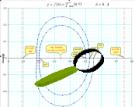
1.6. Very sneaky trajectory with increasing iteration-height
Wrong hypothese in first version: I expected, that, when h diverges to +oo, the spiralling distorts to the shape of a rectangle (dotted red lines) of infinite height, meaning divergence to +/–oo * I .The trajectory shows a much more chaotic behaviour. Far from approximating a rectangle when h->+oo the spiral sneakes around and even tends to encircle the oscillation-points. The plot shows extrema at some heights, so in the near of h=10.5 and h=11.5; I don't know yet, whether we even get infinities there. Also I did not consider the consequences of multivaluedness and/or indeterminacies of fractional powers of negative bases so far.
Graph 3: fractional heights for f(h) approaching heights up to h=14 showing tendency to extremely uneven behave
![]()
1.7. Superlogarithm and trajectory-shortcuts using complex heights
Looking at the trajectory in graph 2 we could ask, whether there is a complex iteration, which allows to proceed directly along the real axis from 0.5 to, say, 0.6 .
Graph 4: directly traverse iterations using complex-valued "heights"? Instead of spiralling along the trajectory of real heights through the complex plane (deep blue spiral trajectory) walk directly on the real-axis(red arrows)
![]()
![]()
![]()
This introduces the need for a logarithm-like function, which determines the "height" of a value, or more precisely, the height-distance between two values. The term "slog" or "superlog" for such a function is fairly well introduced; but since I compute its values by the diagonalization/schröder-function I'll use a distinct name and call this "iteration-height" or simply "height" or "hgh"-function.
The hghb()-function is essentially the log of the schröder-function. The schröder-function expresses increase of iteration-height h by h'th powers of u, in the sense that for a certain height h we have some relation uh -> f(h) and for iteration of an additional height j we have uh*uj = uh+j -> f(h+j) . For the (fixpoint-)unshifted version of the schröder-function we introduce the symbol σ such that for the following we use
σ(x) = s(x') = s(x/t-1)
where s(x') is the function as described above.
The schröder-function has no inherent zero; so it can be/must be normed. For the current article we assign to the value x0=0.5 = f(0) the height h=0. The unnormed schröder-function assigns the value σ(0.5) = 0.478492972731, which is also σ(0.5) = u-0.006176346… + 0.2344679…*I . To have hghb(0.5) = 0 we must normalize
hghb(x) = logu(σ(x)/σ(0.5)) = logu (σ(x)/0.478492972731).
Unfortunately the log is multivalued and especially the attempt to work with a log of a negative base (u~-1.08…) as we do it here cannot supply unambiguous results. However, some first results are quite meaningful.
For instance,
σ(b0.5) = σ(0.2) = –0.519775642476
and
σ(b0.5)/σ(0.5) = –1.08627643894 = u1
thus
hgh(b0.5) = 1
as expected. We find such reasonable results also for heights 0≤h≤1 .
It is more interesting to increase x0=0.5 to x2 = bb0.5~ 0.525305560881 and see, whether we get the expected height-difference 2 this way. But here we run into the ambiguity of logarithms. The computation gives σ(x2)= 0.564620033956 from what
σ(x2)/σ(x0)= 1.17999650180 = u0.001386836 - 0.0526474*I
and the height-value would be
hghb(x2) = log(σ(x2)/σ(x0)) / log(u) = 0.001386836 - 0.0526474*I
thus a complex iteration height to proceed from x0=0.5 to x2~0.5253 directly along the real axis. However, respecting the fact, that x2 is additionally one "winding" around the fixpoint from x0, and inserting 2*π*I in the log-formula for the height we get
hghb(x2) = ( log(σ(x2)/σ(x0)) + 2*π*I ) / log(u) = 2.000 + 0.000*I
which is what we originally expected for the height function.
Gottfried Helms, 26.6.2009
2. Appendix:
2.1. Data for graph of fractional heights
|
h=height |
real(f(h)) |
imag(f(h)) |
|
0.00 |
0.500000 |
0.000000 |
|
0.05 |
0.499530 |
0.023067 |
|
0.10 |
0.496798 |
0.046554 |
|
0.15 |
0.491428 |
0.070735 |
|
0.20 |
0.482719 |
0.095754 |
|
0.25 |
0.469596 |
0.121448 |
|
0.30 |
0.450635 |
0.147015 |
|
0.35 |
0.424374 |
0.170533 |
|
0.40 |
0.390228 |
0.188593 |
|
0.45 |
0.349996 |
0.196871 |
|
0.50 |
0.308675 |
0.192424 |
|
0.55 |
0.272536 |
0.176313 |
|
0.60 |
0.245431 |
0.153238 |
|
0.65 |
0.227361 |
0.128258 |
|
0.70 |
0.216146 |
0.104455 |
|
0.75 |
0.209404 |
0.082918 |
|
0.80 |
0.205374 |
0.063638 |
|
0.85 |
0.202943 |
0.046198 |
|
0.90 |
0.201456 |
0.030094 |
|
0.95 |
0.200541 |
0.014843 |
|
1.00 |
0.200000 |
0.000000 |
|
1.05 |
0.199751 |
-0.014859 |
|
1.10 |
0.199807 |
-0.030168 |
|
1.15 |
0.200289 |
-0.046408 |
|
1.20 |
0.201476 |
-0.064143 |
|
1.25 |
0.203923 |
-0.084044 |
|
1.30 |
0.208680 |
-0.106850 |
|
1.35 |
0.217642 |
-0.133116 |
|
1.40 |
0.233885 |
-0.162445 |
|
1.45 |
0.261201 |
-0.191932 |
|
1.50 |
0.301468 |
-0.214942 |
|
1.55 |
0.350717 |
-0.223578 |
|
1.60 |
0.399740 |
-0.214890 |
|
1.65 |
0.440605 |
-0.192994 |
|
1.70 |
0.470777 |
-0.164536 |
|
1.75 |
0.491598 |
-0.134415 |
|
1.80 |
0.505503 |
-0.105022 |
|
1.85 |
0.514610 |
-0.077095 |
|
1.90 |
0.520398 |
-0.050569 |
|
1.95 |
0.523793 |
-0.025044 |
|
2.00 |
0.525306 |
0.000000 |
|
2.05 |
0.525125 |
0.025135 |
|
2.10 |
0.523155 |
0.050962 |
|
2.15 |
0.518972 |
0.078107 |
|
2.20 |
0.511711 |
0.107180 |
|
2.25 |
0.499848 |
0.138622 |
|
2.30 |
0.480915 |
0.172250 |
|
2.35 |
0.451438 |
0.206211 |
|
2.40 |
0.408086 |
0.235222 |
|
2.45 |
0.351638 |
0.249873 |
|
2.50 |
0.291801 |
0.241753 |
|
2.55 |
0.243192 |
0.213154 |
|
2.60 |
0.212700 |
0.176159 |
|
2.65 |
0.196898 |
0.140931 |
|
2.70 |
0.189623 |
0.111007 |
|
2.75 |
0.186548 |
0.086157 |
|
2.80 |
0.185368 |
0.065165 |
|
2.85 |
0.184967 |
0.046867 |
|
2.90 |
0.184814 |
0.030352 |
|
2.95 |
0.184653 |
0.014918 |
|
3.00 |
0.184355 |
0.000000 |
|
3.05 |
0.183858 |
-0.014908 |
|
3.10 |
0.183143 |
-0.030315 |
|
3.15 |
0.182236 |
-0.046808 |
|
3.20 |
0.181252 |
-0.065137 |
|
3.25 |
0.180506 |
-0.086351 |
|
3.30 |
0.180811 |
-0.111967 |
|
3.35 |
0.184190 |
-0.144066 |
|
3.40 |
0.195404 |
-0.184665 |
|
3.45 |
0.223638 |
-0.232261 |
|
3.50 |
0.278406 |
-0.274413 |
|
3.55 |
0.353681 |
-0.289604 |
|
3.60 |
0.425345 |
-0.270857 |
|
3.65 |
0.476914 |
-0.232520 |
|
3.70 |
0.508842 |
-0.189973 |
|
3.75 |
0.527591 |
-0.150187 |
|
3.80 |
0.538570 |
-0.114657 |
|
3.85 |
0.545088 |
-0.082862 |
|
3.90 |
0.548990 |
-0.053807 |
|
3.95 |
0.551272 |
-0.026492 |
|
4.00 |
0.552437 |
0.000000 |
2.2. Links
Cauchy integral also for b<e(1/e)
http://math.eretrandre.org/tetrationforum/showthread.php?tid=248
Bifurcation of tetration below E^-E
http://math.eretrandre.org/tetrationforum/showthread.php?tid=109
Tetration below 1
http://math.eretrandre.org/tetrationforum/showthread.php?tid=43