Fractional iteration of the function f(x) = 1/(1+x)

Abstract: A self-study exercise in function-iteration

 

In this article I deal with the fractional iteration of a very simple function. We use:

                f(x) = 1 / (1 + x)

and in the iterational notation:

                f°⁰(x) = x
                f°¹(x) = f(x)
                f°^h+1(x) = f°^h(f°¹(x))

The integer iteration for h=0..inf produces the sequence of continued fractions

               

                 (where the bracketed expression denote the infinite continued fraction)

which converges to the golden ratio ~0.618… for all x.

It is not obvious, how to arrive at a formulation which allows interpolation to fractional iterates. We'll see, that such a formulation can be given when the generalization of fibonacci-numbers to fractional and general indexes is introduced, see chap 3. First I use the standard-procedure: rewrite the function as powerseries in x, generate the matrix-operator F; if the powerseries f(x) has a constant term, recenter around a fixpoint t:g(x) = f(x+t)–t , compute the triangular matrix-operator G (the Bell-matrix for functon g(x)) and perform regular iteration by powers of G, where fractional iterates are well defned by fractional powers of G and that fractional powers can be computed using diagonalization:

                G = W *D * W^-1
                G^h = W * D^h * W^-1

where the fractional and general power of the diagoal-matrix D can be implemented by the general power of its scalar diagonal-elements:

                D^h = diag_k=0..inf(d_k,k^h)

 

2.1) f(x) expressed as powerseries

First express f(x) as powerseries

                f(x) = 1 – x + x² – x³ + …  – …

which is the well known expansion.

Caveats: Looking precisely at it, this substitution must be justified; let's consider at least he following:

·         While for the powerseries-expansion of f(x) we know that it must be |x| < 1 for the series to converge, there is no such restriction in the fractional notation. Well, we know that the series can be analytically continued to match the values of the fractional notation – but this indicates that we need some care when we replace one notation by another one.

·         Another discrepancy is the different handling of the domain for the fractional representation vs. the powerseries representation. Under the iteration-aspect this is a more serious aspect; it is for the fractional notation, that the domain thins out the higher the iteration of the fraction is assumed. The domain for 1/(1+x) is IC\{-1}, the domain for 1/(1+1/1+x)) is IC\{-1,-2}, and this continues for each iteration.

Thus: if we want to discuss the iteration of 1/(1+x) depending on the parameter "height" the domain-restriction is somehow part of this function-parameter. I don't have an idea, how this must be discussed for fractional or continuous iteration – maybe the domain is completely thinned out… . However, for the series-representation we don't see such a distinctive characteristic, we only know, that for all |x|>= 1 we have no convergence and must use analytical continuation to allow to extend the domain.

I do not want to go deeper in this here; I assume these problems are solvable and proceed in discussing the properties of the iteration of the powerseries.

2.2) Recentering of f(x): fixpoint-shift to g(x)

The above powerseries f(x) has a constant term and is thus not well suited for fractional iteration. But this may be resolved by reformulation using fixpoint-shift.

The function has two fixpoints x₀ and x₁ which can easily be derived from the fractional representation x = 1/(1+x).

                x = 1/(1+x)                       // definition of a fixpoint for f(x) = x
                x² + x = 1
                x_0,1 + 1/2 = +-sqrt(5)/2
                x₀ = 1/2*(-1+sqrt(5))                   ~ 0.618                                =φ
                x₁ = -1/2*(1+sqrt(5))                   ~ –1.618             = – Φ

                x₀ = 0.618… =  = φ 

 

Then we use the fixpoint to define another function g(x) without constant term

                g(x)       =f(x + x₀) – x₀
                               = –x₀     + 1 – (x+x₀) + (x+x₀)² – (x+x₀)³ + …  – …

Collecting like powers of x and evaluating the series in φ which serve as their coefficients gives, with x₀= φ

                g(x)       =  – φ²x + φ³x² – φ⁴x³ + … –  …     

The function g(x) has now no constant but one nonvanishing linear term, so it can not only be iterated but also be inverted.

2.3) Powerseries-representation and closed forms of f(x) and g(x) and iterates

Also we can proceed to a closed form, since it is also a pure geometric series in (–φx):

                g(x)       =    φ((–φx) + (–φx)² +(–φx)³ + … –  …     
                               =    φ    (–φx )/(1 – (–φx))
                               =  –  φ    (φx )/(1 + φx))

By construction it is also

                f(x)        = g(x – φ)+ φ
                f°²(x)     = g(g(x – φ)+ φ – φ)+ φ
                               = g(g(x – φ))+ φ
                               = g°²(x – φ)+ φ

and the generalization for natural iteration-heights h:

                f°^h(x)     = g°^h(x – φ)+ φ

Since g(x) is invertible, we get even the inverse of g(x) in a closed form:

                g°^-1(x) =  1/( φ + φ²/x ) = 1/φ * 1/( 1 + φ/x )

from where we can crosscheck the inverse of f(x) in its closed form as well.

2.4) Fractional iteration: use of the matrix-method and diagonalization

The iteration and fractional iteration of g(x) is then performed using the associated matrixoperator (a scaled version of the "Bell-matrix") G.

The matrix-operator G has the form

                G             = matrix_r,c=0..inf g_r,c 
                               = matrix_r,c=0..inf (-1)^r φ^r+c *  b_r,c 

                where   for r=0 or c=0                   b_r,0 = b_0,c = 0
                               for r = c = 0                        b_0,0 = 1
                 and       for r,c>0                              b_r,c = binomial(r-1,c-1)

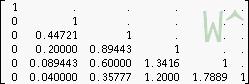
The top left segment of G is (rounded to 6 digits):

G0..5,0..5 =
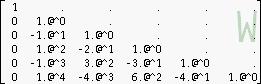
G0..5,0..5 =	Exact, where @ is used for φ

 

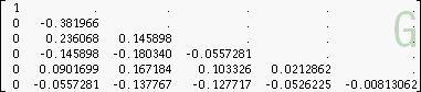
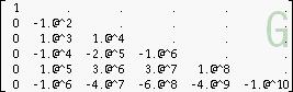
Integer and fractional powers of that matrix will then contain the coefficients for the accordingly iterated function g°^h(x) in its second column. The fractional powers are computed by diagonalization and fractional powers of the matrix-diagonal. Since G is triangular we have finite polynomials in powers of φ only, so we have exact expressions in terms of φ for each coefficient of the powerseries for the fractional iterates.

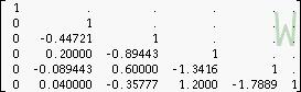
2.5) Diagonalization: G = W * D * W^-1

Diagonalization means, that the matrix G is decomposed in three matrices, where W and W^-1 are lower triangular and D is diagonal. For triangular Bell-matrices like in this case, where the elements of the diagonal are not all powers of 1, this can always be done by a relatively simple procedure, which gives exact coefficients in all tree matrix-factors.

The matrices W, D and W^-1 are (top left segments, matrices have infinite size)

	diag()
Exact, where @ is used for 1/sqrt(5)	Exact, where @ is used for φ	Exact, where @ is used for 1/sqrt(5)
	diag()

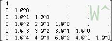
By this construction, W is simply a power of the binomial-matrix ; it is

                W = P ^–1/sqrt(5)                       W^-1 = P ^1/sqrt(5)

Using the rules of diagonalization we can now express powers of G by powers of the diagonalmatrix of eigenvalues D:

                G^h = W * D^h * W ^–1

and precisely we have to write

                G^h = W * diag(_r=0..inf ( d_h^r)) * W^-1

where d_h =(-(φ²))^h must be determined first and of this for each entry in D^h the appropriate integer power is then needed. This care is not needed for iteration to integer heights, but will be needed when continuous iteration with fractional or complex h is attempted.

2.6) Computation of fractional iterates of f(x)

 

Defining a vandermonde-vector V(x) of the general type

                V(x) = rowvector(1, x, x², x³,…)

we have by this

 

                V(x) * G  = V( g(x) )
                                 = V(-φ *   φx /(1 + φx)  )                           //           g(x) = - φ /(1/ (φx) + 1)

the latter functional description using the second column of (the current power of) G.

The same formula serves for general powers of G as discussed in the previous paragraph:

                V(x) * G^h  = V( g°^h(x) )

and introducing the fixpoint-shift:

                V(x–x₀) * G^h  = V( f°^h(x)–x₀ )

2.7) Use of the Schröder-function

Using the diagonalization we have implemented the fractional iteration. But also the matrices W and W^-1 can be seen as the operators for the Schröder-function σ and its inverse σ°^-1 for the function g(x):

                g°^h(x) =   σ°^-1( d ^h  *σ (x))
and
                f°^h(x) =   σ°^-1( d ^h  *σ (x–x₀)) + x₀

Here the cofficients of the Schröder-function are in the second column of W resp. W^-1 and the coefficient d_h is the h'th power of the second entry in the diagonal D:

                σ (x) =

                σ°^-1 (x) =

                d^h = (D_1,1 )^h

 

Then the h'th (continuous) iterate for f(x) can be determined by

 

                f(x)        = g(x – φ) + φ 
                f°^h(x)     = g°^h( x – φ) + φ

                g(x)       = σ °^-1( d(σ (x)))              = σ °^-1( (– φ²) σ (x)))
                g°^h(x)   = σ °^-1( d°^h(σ (x)))           = σ °^-1( (– φ²)^h σ (x)))

                f°^h(x)     = σ °^-1((– φ²)^h (σ (x– φ ))) + φ

Since the Schröder-funtions are again geometric series, we can give closed forms for them:

                σ (x)      =x sqrt(5) /( sqrt(5) + x )
                σ°^-1(x)   = x sqrt(5)/( sqrt(5) – x)

and can determine exact coefficients in terms of powers of φ .

 

2.8) Observations/Questions

We noticed, that the second eigenvalue of the matrix G is negative; so fractional powers require complex values for the diagonal, and thus, by this method, we get complex values for real fractional iterates of real initial values.

I'd like to see possibly concurring methods to compare the results here.

Below are some plots for fractional iterates for h=0 to 2 in steps of 1/10 for the initial values x=1 and x=0.25.

Questions:

·         is there a concuring method for fractional iteration? What values does it produce

·         how can we express the function using the second fixpoint for fixpoint-shift according to the above rationale

 

Gottfried Helms; 28.01.2009

Update 10'2009: I could give an aswer to the first question myself. See next chapter.

If we look at the coefficients of the fraction when integer-iterated, we notice the progression related to the fibonacci-numbers.

               

which is not difficult to show in generality by induction. Now there is a continuous extension for the fibonacci-numbers, such that we can use fibonacci-numbers of fractional and finally of arbitrary complex index. The formula for a function, containing the height-parameter h as well reads

               

where

               

and

               

Writing for a constant argument x (for instance x=1) a new function depending only on h:

                fh(h) = f°^h(1)

we get the same values and the same plot as in the previous chapter. See appendices.

Gottfried Helms; 5.10.2009

 

4.1) f(f(x)) as smoothed function, which has real fractional iterates

Since the second eigenvalue of G is negative, iterates of f(x) produce this spiraling behaviour when iterated in noninteger stepwidth (see plot "pic 1"). 

If we use ff(x) = f(f(x)) as iterable function, then its second eigenvalue is positive and there should be a fractional iteration giving a real trajectory only.

We have for ff(x) and the inverse ff°^-1(x) the definitions:

               

Since ff(x) has a positive eigenvalue, we can find a half-iterate which has also a positive eigenvalue, again using fixpoint-shift by φ. Call the fixpoint-shifted version of ff(x)gg(x), such that ff(x) = gg(x+ φ )– φ  . Call the half-iterate of gg(x)gg°^0.5(x), where I found the analytic description of the coefficients heuristically (and they are not proven correct). Assume the correctness, then for the half-iterate of ff(x) we get:

               

finally

(1)        

 

which provides meaningful results, if we, for instance start with x=1, compute x₁=ff°^0.5(x) , x₂=ff°^0.5(x₁) and see that the results match: x₂ = ff(x) . Also the taylor-coefficients of ff(x) and ff°^0.5(ff°^0.5(x)) come out to be equal as far as checkable by Pari/Gp, and finally, using the symbolic algebra-system Maxima, we simplify using the definition (1):

                ff°^0.5(ff°^0.5(x)) = (1+x)/(2+x)

which is the expected result

4.2) ff(x) as iteration-series

If I want to express a function f(x) as a series of iterates of a function ft(x) (let's call this an "iteration-series", I used "powertowerseries" in context of tetration here), then we have the following relation for a possible definition of ft(x):

                K + x + ft(x) + ft°²(x) +  ft°³(x) + …          = f( x )
                K +       ft(x) + ft°²(x) +  ft°³(x) + …           = f( ft(x) )

                x                             = f( x ) – f( ft( x ) )
                f( ft( x ) )             = f( x ) –   x
                ft( x )                    = f°^-1( f( x ) – x )

Inserting ff(x) and ff°^-1(x) here for f we get for ft( x )

               

or as taylorseries

               

It can also be described by the strange representation:

               

The trajectory of iterates of ft(x) is very chaotic and seems to not to converge in a classical sense.

Fixpoints:

               

The fixpoints are x₀=0, x₁,x₂=-2 , one quadratic singularity at x=-1

(see a plot at pic 5 below)

Pic 1:

Trajectories for fractional iteration f°^h(x) for two initial values x:

 

Pic 2:

The vectorial angles between coordinates of iterates and the coordinate of the limit [φ,0*î] taken as origin are nearly equal, the angle is nearly a linear function of the iteration-height h

 

Pic 3:

The complex coordinates on the trajectory for x=1 can be translated moving the origin to the limit-point [φ,0*î] = [0.6183…,0*î] on the real axis. Then the angles of the vectors from origin to the points are approximately equi-angular. Use for convenience the notation fh(h) instead of f°^h(1) in the following.

Here the lengthes (abs(fh(h)– φ) ;blue line) and the angles (arg(fh(h)– φ)/Pi  ;magenta line) for the points, when the origin is translated to [φ,0*î]:

The magenta line for the angles is nearly linear. In the following picture the deviation from linearity (the non-equi-angularity) of the trajectory is shown.

Pic 4:

Where the sinusoidal curve meets the x-axis, the trajectory(magenta line) meets the y=x-line. We see the slightly distorted deviation from a straight line which is visually magnified by a rescaling-factor of about 200 and shown with the red sinusoidal curve.

 

Pic 5 (see: loose ends)

The (cobweb-) trajectory of the function ft(x), where

                ff(x) = x + ft (x) + ft^°2 (x) + ft^°3 (x) + …     = (x+1)/(x+2)

 

 

by powerseries f°h(0.25)

by powerseries f°h(1)

by fib–interpolation fh(h)

 

h	real	imag		real	imag		real	imag
0	0.25000	0.00000		1.00000	0.00000		1.00000	0.00000
0.1	0.28858	-0.09009		0.93487	0.11961		0.93487	0.11961
0.2	0.34421	-0.16567		0.84412	0.19296		0.84412	0.19296
0.3	0.41497	-0.22339		0.75041	0.22383		0.75041	0.22383
0.4	0.49737	-0.25899		0.66712	0.22259		0.66712	0.22259
0.5	0.58537	-0.26829		0.60000	0.20000		0.60000	0.20000
0.6	0.67002	-0.24917		0.55033	0.16472		0.55033	0.16472
0.7	0.74074	-0.20370		0.51727	0.12311		0.51727	0.12311
0.8	0.78815	-0.13931		0.49915	0.07971		0.49915	0.07971
0.9	0.80744	-0.06741		0.49407	0.03784		0.49407	0.03784
1	0.80000	0.00000		0.50000	0.00000		0.50000	0.00000
1.1	0.77227	0.05400		0.51486	-0.03183		0.51486	-0.03183
1.2	0.73280	0.09031		0.53639	-0.05613		0.53639	-0.05613
1.3	0.68954	0.10886		0.56210	-0.07188		0.56210	-0.07188
1.4	0.64844	0.11216		0.58933	-0.07869		0.58933	-0.07869
1.5	0.61321	0.10377		0.61538	-0.07692		0.61538	-0.07692
1.6	0.58576	0.08740		0.63782	-0.06777		0.63782	-0.06777
1.7	0.56671	0.06632		0.65477	-0.05313		0.65477	-0.05313
1.8	0.55586	0.04330		0.66516	-0.03537		0.66516	-0.03537
1.9	0.55250	0.02061		0.66889	-0.01694		0.66889	-0.01694
2	0.55556	0.00000		0.66667	0.00000		0.66667	0.00000

 

 

Comparision 1

Cite (a formatting and replacement of symbols):

Von:                    Matt matt271829-news@yahoo.co.uk
Datum:               Thu, 22 Jan 2009 14:00:23 -0800 (PST)
Nachricht-ID:    <062e3101-0350-4540-86bc-3ccafb73daf9@v18g2000pro.googlegroups.com>

            Some while ago, when I was playing with this, I got, for the more general

                           f(x) = 1/(a*x + b),

 

                                                                 (ax + b - β)* α ^{n - 1} – (ax + b - α)* β^{n - 1}
                              f°ⁿ(x)                 = ---------------------------------------------------
                                                                  (ax + b - β)* αⁿ    – (ax + b - α)* βⁿ

where
                              α = (b + Sqrt(b² + 4*a))/2
                              β = (b – Sqrt(b² + 4*a))/2

Since

                               b – β = b – b/2 + Sqrt(b² + 4*a)/2 = b/2 + Sqrt(b² + 4*a)/2 = α
                               b – α = b – b/2 – Sqrt(b² + 4*a)/2 = b/2 – Sqrt(b² + 4*a)/2 = β 

the above simplifies and gives

                                                                     (ax + α)* α ^n–1 – (ax + β)* β^n–1     
                                  f°ⁿ(x)                 = ------------------------------------------ -
                                                                      (ax + α)* αⁿ    – (ax + β)* βⁿ

For a=b=1 this reduces to

                                                                     (x + α)* α ^n–1 – (x + β)* β^n–1     
                                  f°ⁿ(x)                 = ------------------------------------------ -
                                                                      (x + α)* αⁿ    – (x + β)* βⁿ         

                               where                 

The computation gives the same result as my method.

(Update 4.10.2009: this ssems to be the same as the method using interpolated fibonacci-numbers)

Comparision 2:

Using φ=(sqrt(5)-1)/2  the fractional iterate (with initial value x=1) dependend on h can be expressed as

               

or, using

               

and converting the sum (which is a geometric series) into the closed form, gives

               

This method gives the same values as the original method.

 

I formatted the following usenet-post for better readability here. The author may please forgive…

Von:                    alainverghote@gmail.com
Datum:               Fri, 23 Jan 2009 02:58:41 -0800 (PST)
Nachricht-ID:    <e2e35fd7-48c7-4843-89bf-53f6a6b919e8@o40g2000prn.googlegroups.com>

Good morning,

 

The problem of continuous iteration (ax +b)/(cx +d) is simply solved:

from a direct classification according to the number of fixed points:
            zero,
            one,
            two,
            infinity

and
            pole or not.

 

Here:    h(x) =1/(1+x) has two fixed points 

                           x₁ = (-1+sqrt(5))/2                       x₂ = (-1-sqrt(5))/2

            and a pole
                           x =-1

 

May be written

            (h(x)-x₁)/(h(x)-x₂)        =  a*(x–x₁)/(x–x₂)
            for x = 0 ,h(0) = 1   then a = (1+sqrt(5))/(1–sqrt(5))

 

And also

            (h° ⁿ(x) – x₁)/(h° ⁿ(x) – x₂)         = aⁿ *(x – x₁)/(x – x₂)

 

just mind 'a'  is real negative!

Alain

 

Of course there are known solutions in term of matrices, I only show there exist other ways, we might also use Ad Hoc parametrization

 

Example:

            x(t) = 1+2/t,
            t =>t +3  or
             h(x(t))= 1 +2/(t+3)

            h°^[r](x(t)) = x(t+3*r) 

corresponds to

            h(x)=(5x - 3)/(3x - 1)

and directly we've got

            h°^[r](x)=((3r+2)x – 3r)/(3rx + 2 – r)

All homographic functions h(x) can be parametrized,

Ex.

            h(x)=1/(1+x)
            x =f(t) =(1+sqrt(5)-t*(1-sqrt(5))/2 ,

            t=> a*t ,
            a = ((1+sqrt(5))/(1-sqrt(5))
            h(x)=h(f(t))=f(a*t)

And an interesting property :

            h°^[r](x) = h°^[r](f(t)) = f(a^r*t),

 

Gottfried Helms; 5.10.2009      
(previous versions: 23.01.2009)