Tetration Gottfried Helms - Univ Kassel            07' 2007 - 2008

 

 

 

 

Version 2.1

Gottfried Helms, 31.12.2008

 

 

Recently in the tetration-forum, H. Trappmann proposed in [TForum] a binomial-method for definition of fractional tetration. The basic binomial formula can also be found in [Woon] and in [Comtet], where the authors used it in a context of matrix-notation. Here it was applied directly to the function-values, thus giving an example of application of a "powertower-series". The following formula is valid also for fractional  iteration-"heights" h:

(1)

f°h(x) =

"Bin-Ex"-formula

 

This method has some special flair. First, it is valid for general functions, thus not only for powerseries. Second, we need only integer iterates of the function, and combine it with the well known and arbitrarily precise computable gamma-function involving the fractional parameter h.                   
For tetration we may say: we translate a problem which is usually formulated as a problem of powerseries into one of a powertowerseries. For me this is principally a very interesting aspect; further alternative candidates for the representation of the fractional powertower were for instance Julia- and Noether-series, but I've not yet seen a discussion of this possibility.

In the following I show the relation between the binomial-approach and the diagonalization and the "exponential polynomial interpolation"[Helms], which thus seem to give identical results, at least as far as convergence is given.

 

 

 

The results computed via the binomial-method were well approximated by that via diagonalization in an earlier treatise [Tforum1]; actually it occured that the diagonalization gave better approximated results much faster (using less terms getting better approximation) than the binomial-method, and the results for both methods are identical only in the limit where infinitely many terms of the series are involved.

However, to compare those results more rigorously needs to show the equivalence analytically. I'm not yet able to do that. But what I can do is to compare the methods when the integer powertowers of the binomial-method are expressed as powerseries of integer heights – where there is no controversy about the correctness of all solutions under discussion.

Application of the given binomial formula to the coefficients of the formal powerseries for integer heights leads to the following-formulae, expressed in my matrix-notation for brevity.

First the matrix-notation for the computation of a powertower of heights 1,2,3,...:

                V(x)~ * U_t  [,1]                  = U_t(x)                  // the brackets [,1] mean extraction of 2^nd column, the
                V(x)~ * (U_t)²[,1]               = U_t°²(x)               //   rhs is the scalar value of the function U()
                V(x)~ * (U_t)³[,1]               = U_t°³(x)
                ...

Collect all the above second columns of the powers of U_t into a (list)-matrix LIST:

(2)          LIST = [ (U_t)⁰[,1],     U_t [,1],    (U_t)²[,1] ,  (U_t)³[,1], ...  ] 

Then obviously the matrix-product

(3)          V(x)~ * LIST        = [ U_t°⁰(x),    U_t°¹(x),    U_t°²(x) ,  U_t°³(x), ...  ]
                                               = [        x  ,      U_t(x),    U_t°²(x) ,  U_t°³(x), ...  ]
                                               = PT(x)~

gives the consecutive iterates/powertowers of the function U_t(x) in a resulting rowvector PT.

This resembles the

-part in the above BinEx - formula (1)

 

These iterates should now first be composed using the signed binomial-coefficients, which means in matrix-notation:

(4)          PT(x)~ * P^-1 ~ = PT₁(x)~

This resembles the

-part in the above BinEx - formula (1)

 

Then the binomial-coefficients for the fractional exponent h shall be used for the final step of composition. Call the columnvector containing these BIN_h. The dot-product of PT₁ and BIN_h gives then the scalar result:

(5)          PT₁(x)~ * BIN_h = U_t°^h(x)

This finally resembles the

-part in the above BinEx - formula (1)

 

 

 

As shown in the article "exponential polynomial interpolation" I found, that the matrix LIST can be decomposed into two matrix-factors Poly and VV (where also Poly can be expressed as composition of parts of the diagonalization-matrices W^-1 and W). This allows to rewrite the whole operation as a matrix-formula and to observe the identity of the different methods:

                V(x)~ * LIST * P^-1~ * BIN_h
                                               // LIST containing the coefficients of powerseries for consecutive integer
                                               //      heights
                                               // BIN_h the column-vector containing the fractional binomials

Now the decomposition of LIST into its factors is used:

                V(x)~ * (Poly * VV(u^k) ) * P^-1~ * BIN_h     
                                               // factor LIST into the polynomials and matrix VV of arguments
                                               // Here rows and columns in VV are Vandermonde-vectors which is
                                               // crucial for the simple proof of the method-identity

Since the rows in VV are vandermonde, the rightmultiplication by P^-1~ is a simple application of the binomial-theorem. We exploit associativity of matrix-multiplication (since all involved products are finite sums) and rewrite this product first:

                V(x)~ * Poly * (VV(u^k)  * P^-1~ )* BIN_h      // using matrix-associativity
                V(x)~ * Poly * (VV(u^k-1) * BIN_h )                              // applying binomial-theorem to rowvectors

 

Now the next rightmultiplication is another application of the binomial-theorem (for fractional powers) and since BIN_h is a column-vector only, the result is also a columnvector:

                V(x)~ * Poly * V((1+u-1)^h)                           // application of binomial theorem
                V(x)~ * Poly * V(u^h) = U_t^°h(x)                      // yields identity with "exponential polynomial interpolation"
                                                                                              // and diagonalization-formula

The last formula is exactly the same which we would get, if we used the "exponential polynomial interpolation" method. It is even identical to the result of the diagonalization procedure if we adapt order of computation:

                V(x)~ * U_t^h         = V(x)~ * (W^-1 * ^dV(u^h) *W )                        // diagonalization-formula

Here, since we need only the second column of W for the value of the function, we can write

                V(x)~ * U_t^h [,1]  = V(x)~ * W^-1 * ^dV(u^h) *W [,1] 
                                               = V(x)~  * (W^-1 * diag(W [,1])) *  V(u^h)

where the parenthese is equal to the previous matrix Poly, so we get the same result as before:

                V(x)~ * U_t^h [,1]  = V(x)~  * Poly *  V(u^h)

and the methods are equal except of the order of summation and thus of the position, where the truncation-error occurs due to computations with only finitely many terms.

 

\\ Pari/GP using PariTTY-interface © Gottfried Helms
\\ ("%"-commands are expanded or redirections of output

n=32                               \\ set global matrixsize
\r % _matrixinit.gp                \\ initialize standard-matrix-functions

[u=0.5,t=exp(u),b=exp(u/t)]        \\ parameters to work with, b not used here

Ut = dV(u)*fS2F;                   \\ constructing from Stirling-numbers 2^nd kind

    \\ create list-matrix for coefficients of powerseries of integral heights
UtList = matrix(n,n);             
tmp = 1.0*matid(n);for(k=1,n,UtList[,k]=tmp[,2];tmp=tmp*Ut);

%box >UtList UtList        \\ list contains powerseries for consecutive heights

\\ set parameters for problem
x = 1.0
h = 0.5                            \\ height = 0.5

%box >PT V(x)~ * UtList            \\ check the computation of powertowers
Ut1 = UtList*PInv~                 \\ Pinv is inverse of binomial-matrix
BM = Ut1*matrix(n,1,r,c,binomial(h,r-1)    \\ BM is resulting col-vector
print (V(x)~ * BM)                 \\ check approximative result

            \\ diagonalization into matrices 2,3 and 4 of the array UtKenn
UtKenn = APT_Init2EW(Ut);          \\ initialize diagonalization-matrices
POLY = UtKenn[2]*matdiagonal(UtKenn[4][,2]) \\ create POLY-matrix
UtTerms05 = POLY * Mat(V(u^h))     \\ create coeffs for diag-solution with height h
%box >POLYSol V(x)~*POLY * Mat(V(u^h))
%box >DIAGSol V(x)~* UtTerms05

\\ show differences of coefficients of binomial- and diagonalization method
\\ show results when increasing terms of fractional binomial-formula
MCompare=matrix(n,n,r,c,sum(k=1,c,Ut1[r,k]*binomial(h,k-1) – UtTerms05[r,1]))
%box >compare MCompare ~           \\ should asymptotically (greater dimension n)
                                   \\ approximate zero-difference

Increasing rownumber means increasing number of used terms; the columns display the coefficients at powers of x – always difference between binomially – computed terms and diagonalization-computed terms (n=1..32)

*x0	*x1	*x2	*x3	*x4	*x5	*x6	*x7	*x8
0	2.9289E-1	-1.0355E-1	-5.3441E-3	1.2433E-4	-2.0154E-5	-3.9712E-6	1.2467E-6	1.2640E-7
0	4.2893E-2	-4.1053E-2	5.0726E-3	1.4264E-3	1.1005E-4	6.8795E-6	2.0217E-6	1.7484E-7
0	1.1643E-2	-2.1522E-2	6.7002E-3	1.0805E-3	-8.6276E-5	-5.2926E-5	-1.3181E-5	-3.3916E-6
0	3.8307E-3	-1.2245E-2	6.5170E-3	5.2678E-4	-2.7458E-4	-9.5010E-5	-1.9375E-5	-3.3227E-6
0	1.3893E-3	-7.2857E-3	5.7938E-3	1.4355E-5	-4.0652E-4	-1.1094E-4	-1.5833E-5	-1.1185E-8
0	5.3482E-4	-4.4685E-3	4.9526E-3	-3.9657E-4	-4.8047E-4	-1.0487E-4	-5.2944E-6	5.2159E-6
0	2.1439E-4	-2.8038E-3	4.1497E-3	-7.0172E-4	-5.0663E-4	-8.3221E-5	9.2534E-6	1.1127E-5
0	8.8501E-5	-1.7913E-3	3.4395E-3	-9.1439E-4	-4.9707E-4	-5.1920E-5	2.5364E-5	1.6802E-5
0	3.7360E-5	-1.1615E-3	2.8339E-3	-1.0520E-3	-4.6260E-4	-1.5681E-5	4.1258E-5	2.1637E-5
0	1.6051E-5	-7.6258E-4	2.3276E-3	-1.1312E-3	-4.1199E-4	2.2015E-5	5.5747E-5	2.5282E-5
0	6.9952E-6	-5.0600E-4	1.9090E-3	-1.1663E-3	-3.5193E-4	5.8744E-5	6.8111E-5	2.7580E-5
0	3.0845E-6	-3.3883E-4	1.5652E-3	-1.1689E-3	-2.8740E-4	9.2906E-5	7.7975E-5	2.8507E-5
0	1.3736E-6	-2.2869E-4	1.2837E-3	-1.1482E-3	-2.2195E-4	1.2353E-4	8.5210E-5	2.8127E-5
0	6.1690E-7	-1.5543E-4	1.0537E-3	-1.1111E-3	-1.5804E-4	1.5010E-4	8.9857E-5	2.6560E-5
0	2.7907E-7	-1.0629E-4	8.6580E-4	-1.0633E-3	-9.7319E-5	1.7243E-4	9.2063E-5	2.3956E-5
0	1.2705E-7	-7.3078E-5	7.1234E-4	-1.0087E-3	-4.0808E-5	1.9054E-4	9.2043E-5	2.0477E-5
0	5.8163E-8	-5.0489E-5	5.8688E-4	-9.5034E-4	1.0909E-5	2.0460E-4	9.0046E-5	1.6290E-5
0	2.6759E-8	-3.5034E-5	4.8423E-4	-8.9050E-4	5.7572E-5	2.1490E-4	8.6334E-5	1.1551E-5
0	1.2365E-8	-2.4405E-5	4.0012E-4	-8.3077E-4	9.9147E-5	2.2174E-4	8.1170E-5	6.4096E-6
0	5.7368E-9	-1.7061E-5	3.3111E-4	-7.7228E-4	1.3575E-4	2.2549E-4	7.4804E-5	9.9845E-7
0	2.6711E-9	-1.1966E-5	2.7440E-4	-7.1583E-4	1.6762E-4	2.2648E-4	6.7471E-5	-4.5627E-6
0	1.2478E-9	-8.4168E-6	2.2774E-4	-6.6192E-4	1.9502E-4	2.2507E-4	5.9387E-5	-1.0169E-5
0	5.8459E-10	-5.9363E-6	1.8928E-4	-6.1087E-4	2.1829E-4	2.2158E-4	5.0746E-5	-1.5732E-5
0	2.7464E-10	-4.1972E-6	1.5753E-4	-5.6285E-4	2.3777E-4	2.1632E-4	4.1721E-5	-2.1175E-5
0	1.2935E-10	-2.9743E-6	1.3129E-4	-5.1791E-4	2.5380E-4	2.0958E-4	3.2462E-5	-2.6435E-5
0	6.1058E-11	-2.1122E-6	1.0955E-4	-4.7603E-4	2.6671E-4	2.0161E-4	2.3102E-5	-3.1461E-5
0	2.8884E-11	-1.5029E-6	9.1534E-5	-4.3715E-4	2.7682E-4	1.9265E-4	1.3753E-5	-3.6211E-5
0	1.3691E-11	-1.0713E-6	7.6571E-5	-4.0115E-4	2.8443E-4	1.8290E-4	4.5124E-6	-4.0654E-5
0	6.5017E-12	-7.6496E-7	6.4128E-5	-3.6790E-4	2.8984E-4	1.7254E-4	-4.5408E-6	-4.4767E-5
0	3.0928E-12	-5.4707E-7	5.3768E-5	-3.3724E-4	2.9329E-4	1.6174E-4	-1.3340E-5	-4.8533E-5
0	1.4736E-12	-3.9183E-7	4.5130E-5	-3.0901E-4	2.9503E-4	1.5065E-4	-2.1830E-5	-5.1942E-5
0	7.0317E-13	-2.8103E-7	3.7919E-5	-2.8307E-4	2.9527E-4	1.3938E-4	-2.9968E-5	-5.4989E-5

 

It is interesting, that the leading terms (at low powers of x) show good improving approximations, but the terms at higher powers of x are worse approximated. However, the analytically applied binomial-formulae (implying infinitely many terms) give the same result as the diagonalization (which are exact since the involved matrices are triangular)

 

Gottfried Helms, Aug 2008 (last edit 5.12.2008)

 

For U-tetration the matrices U and U_tare the triangular Stirling-matrix scaled as the following:

            U = ^dF^-1*S2 * ^dF                       // performs x - >exp(x)-1
            U_t = ^dV(u)* U                          // where u=log(t); performs x -> t^x – 1

where the involved (infinite size assumed) matrices are (only the top-left segment is displayed):

 

V(u) =             dV(u) = diag(V(u))	columnvector([1, u, u2,u3,u4,...]) diagonal arrangement
dF =	diag(0!,1!,2!,3!,...)
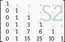
S2 =	Stirlingnumbers 2nd kind
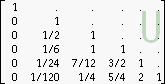
dF-1*S2 * dF = U =
Ut = dV(u) * U =	the numerical value for u=log(t) is actually used here

 

Note: the related "Bell"-matrix for the exponential-function is just another convention to use U_t: it is a similarity-scaling of U_t, where the factorials are removed and assigned to the Vf(x)=[1, x/1!, x²/2!, x³/3!,…]-vector:

                BELL_t = ^dV(u) * S2 = ^dF U ^dF^-1                       // BELL-matrix for function exp(x)-1
then:
                V(x)~ * U_t = V(t^x-1)~
                V(x)~* (^dF^-1 * ^dF) U_t ^dF^-1 = V(t^x-1)~ ^dF^-1
                (V(x)~* ^dF^-1) * (^dF U_t ^dF^-1 ) = (V(t^x-1)~ ^dF^-1 )
                Vf(x)~  * BELL_t = Vf(t^x-1)~

The "Carleman"-matrix is the transposed of the "Bell"-matrix.

In a letter in the tetration-forum I compared numerically the approximation of one T_b°⁰⁵(1) – example using the diagonalization method and the binomial-expansion-method. To have best convergence/comparability in both methods I use b=sqrt(2) as base, so we discuss here the half-integer iteration of the base-function, using x=1:

                T_b(x) := sqrt(2)^x
                T_b^°1(x) := T_b(x)                   T_b^°h+1(x) := T_b^°h(T_b(x))                      T_b^°0(x) = x

or, in a more common tetration-notation

                T_b^°0.5(1) :=  sqrt(2)^{^^0.5}

The binomial-expansion method (BinEx-method) needs many terms for acceptable approximation; for instance, if I even proceeded from using 90 to 96 terms the result had not yet stabilized for more than a handful significant digits.

However, the convergence can be improved when one does not compute the half-integer iterate h=0.5 but for instance h=5.5 or even h=15.5 – convergence to a final result occurs with much less terms. On the other hand, the result for h=15.5 can be reduced by logarithmizing, since taking the logarithm of the result simply decreases the height by 1; and taking the logarithm, even repeatedly, can be performed with arbitrary accuracy.

So I computed

                y_k = T_b°^0.5+k (1)                                   // using BinEx-method
                T_b°^0.5(1) = T_b °^-k(y_k)                          // using logarithm-function to base sqrt(2)

for various k and compared this with diagonalization-method (which employs also the fixpoint-shift by fp=2 and the replacement by the U_t-function):

                T_b °^0.5(x) = V(x-2)~ * U₂^0.5 [,1] +2                                              // using diagonalization

The value, which I computed using diagonalization is obviously verified as far as possible in this numerical computation (and seems also to be the best approximation, see below)

Here is an overview over the quality of approximation, using differently many terms (each subsequent line shows the result, computed with one more term). Also, since T_b°^h(1) for b=sqrt(2) converges to 2 for h-> inf , the columns for h=7.5,8.5,9.5 show the approximation to a value near 2, of which the logarithm must then be taken k-times repeatedly to get the final value (see next table):

 

Table A2.1) of partial sums of series for y_k = T_b°^k+0.5(1), T_b(x)= sqrt(2)^x

                                                                              (using also a small order of Euler-summation)

We see the improvement of convergence to a final value in the columns for higher k.

 

In the following table I compare the results for T_b°^0.5(1) of the above table when the final k-fold application of logarithmizing is included. We see that the accuracy – in terms of reliable digits – improves significantly with higher k:

Table A2.2)  for T_b°^0.5(1) computed by T_b°^-k(y_k)

 

Another interesting aspect is, that the approximants actually appear as narrowing intervals. See the table below, where the above approximants are differently ordered. Note also the remarkable result that the value, which was found with the diagonalization-method

                computed by diagonalization method (by U_t-conversion using fixpoint 2)

is precisely in the middle of the smallest interval found with the BinEx-method:

This result strongly suggests the asymptotic equivalence of the two methods, where for the BinEx-method we either need many more terms for the original problem, or need a very high k-value for the forward/back-transformation into a problem with greater height-parameter h.

Here are the first 64 terms for the series for the tetration to base b=2^1/2 computed by the diagonalization-method, where also fixedpoint shift was applied. I'm using u=log(2) in the notation:

                sqrt(2)^{^^h} = exp_sqrt(2)°^h(1) = a₀ + a₁ u^h + a₂ u^2h + a₃ u^3h + …

= 2

-0.632098661050829250355450645991*(u^h)

-0.225634285681136516413143425561*(u^h)^2

-0.0854081730269597594499116928499*(u^h)^3

-0.0335771160754674029230001663424*(u^h)^4

-0.0135675339902202147608494859091*(u^h)^5

-0.00559920683945879327893257129096*(u^h)^6

-0.00235003288784603927509606731220*(u^h)^7

-0.00100003647234511530676848421238*(u^h)^8

-0.000430480708304067129852499493291*(u^h)^9

-0.000187116458671486711283152071503*(u^h)^10

-0.0000820114021745124653730621286010*(u^h)^11

-0.0000362027647360033178552438925892*(u^h)^12

-0.0000160807242165032926991720492216*(u^h)^13

-0.00000718169500163987888381992083542*(u^h)^14

-0.00000322271898337829632971587206700*(u^h)^15

-0.00000145228984160778882339118309085*(u^h)^16

-0.000000656926890185867110992269509415*(u^h)^17

-0.000000298154140684170905249756457142*(u^h)^18

-0.000000135730176452735916575436728163*(u^h)^19

-0.0000000619577730720144525263961992892*(u^h)^20

-0.0000000283522848886595327370420402643*(u^h)^21

-0.0000000130033888474150892926488383897*(u^h)^22

-0.00000000597608342583576065547607509998*(u^h)^23

-0.00000000275165501558503340886138117415*(u^h)^24

-0.00000000126917896343946963926837959766*(u^h)^25

-0.000000000586333973927660351624141676737*(u^h)^26

-0.000000000271274348008122776988357651664*(u^h)^27

-1.25680399976761153161588768795E-10*(u^h)^28

-5.83015364710942207487235606316E-11*(u^h)^29

-2.70775077829939341682012474069E-11*(u^h)^30

-1.25898302876856412891387370532E-11*(u^h)^31

-5.85980274638521230654861745694E-12*(u^h)^32

-2.73004804447318672548212131442E-12*(u^h)^33

-1.27308225172530456855707356943E-12*(u^h)^34

-5.94180528490971870298055223590E-13*(u^h)^35

-2.77546010867650569889478146944E-13*(u^h)^36

-1.29743844620268719176948000292E-13*(u^h)^37

-6.06954120087079879363699874937E-14*(u^h)^38

-2.84135704644481727983425598351E-14*(u^h)^39

-1.33101016724942278184923950005E-14*(u^h)^40

-6.23890605947345001719322322923E-15*(u^h)^41

-2.92613222099120822272775828837E-15*(u^h)^42

-1.37317444092107054423740563640E-15*(u^h)^43

-6.44751584221885914155573852473E-16*(u^h)^44

-3.02889003575352596475661415485E-16*(u^h)^45

-1.42360371708489474738306639904E-16*(u^h)^46

-6.69422046153196267455087923288E-17*(u^h)^47

-3.14925302230598906034154840721E-17*(u^h)^48

-1.48218916813490386899594957320E-17*(u^h)^49

-6.97879808914843084907249219984E-18*(u^h)^50

-3.28723978294155322857441693926E-18*(u^h)^51

-1.54899187254952507035663848621E-18*(u^h)^52

-7.30175968485491625580317974418E-19*(u^h)^53

-3.44318666249048695192497005860E-19*(u^h)^54

-1.62421142055847837710917189907E-19*(u^h)^55

-7.66422321069973473621175018960E-20*(u^h)^56

-3.61769740197441776246979488582E-20*(u^h)^57

-1.70816579930374362260368051277E-20*(u^h)^58

-8.06783348848322283099536937014E-21*(u^h)^59

-3.81161133353678049861942748125E-21*(u^h)^60

-1.80127883913901077505787760370E-21*(u^h)^61

-8.51471301262827628292471852367E-22*(u^h)^62

-4.02598429898193824724121200470E-22*(u^h)^63

- …

 

[TForum]        Henryk Trappmann
matrix function like iteration without power series expansion
http://math.eretrandre.org/tetrationforum/showthread.php?tid=186
(Henryk Trappmann et al.): mainpage at: tetration-forum

[Tforum1]       Trappmann/Robbins et al.
Parabolic iteration
http://math.eretrandre.org/tetrationforum/showthread.php?tid=11&pid=26#pid26

[Comtet]        Louis Comtet
Advanced Combinatorics
D. Reidel Publishing Company; Dordrecht, Holland; 1970.
pages 144-148

[Woon]          S.C.Woon
Analytic Continuation of Operators — Operators acting complex s-times
arXiv:hep-th/9707206 v2 31 Jul 1997

from my list of explorative articles

[Helms]           Gottfried Helms
exponential polynomial interpolation
http://go.helms-net.de/math/tetdocs/ExponentialPolynomialInterpolation.pdf

Project-index:

[Index]           Gottfried Helms, technical articles on Tetration