Tetration     Gottfried Helms - Univ Kassel          04 - 2008

 

 

Powerseries for U_t at fractional heights

Coefficients of powerseries for fractional iteration U_t^oh(x)

 

Abstract:

Iteration of the function U_t(x) = t^x–1 to fractional heights provides powerseries, whose coefficients mostly strongly diverge and oscillate. I.N. Baker proved in [Bak], that fractional iterates of the function exp(x) – 1 have convergence-radius zero and thus cannot conventionally be summed. The divergence and irregular oscillating of signs is so nasty, that even common techniques for divergent summation like Cesaro- and Euler-sum give no satisfying result - if their results are usable at all.

Here I give a graphical overview in three examples of different characteristics, for bases t=2, t=3, and t=exp(2) .

[Update:]

It seems, that a new series-transformation using the Stirlingnumbers 2^nd kind is suitable to convert the powerseries with diverging coefficients into such of convergent coefficients – thus an expanding of the range of convergence for x from zero to finite values is now realized (hopefully to infinity, must be proven). See chap 3.

Gottfried Helms, D-Kassel       Ver 2.2; 6.02.09

1.      Definitions

1.1.       Definition of the base-function U_t(x) and U_t^oh(x)

2.      Plots

2.1.       Base t=exp(2) ~ 7.3891

2.2.       Base t = 3

2.3.       Base t = 2

3.      Achieving convergence by Stirling-transformation

3.1.       Base t=exp(2) ~ 7.3891

3.2.       Base t=exp(3) ~ 20.086

3.2.1.         First power of U

3.2.2.         Using second power, U²

3.2.3.         Using third power, U³

3.2.4.         Hypothese

3.3.       Results

3.4.       Provisorial conclusion / Impulse to proceed

4.      Appendix

4.1.       Matrix-definitions

4.2.       Tables

4.2.1.         Base t=exp(2)

5.      References

 

 

Define the iterable function

            U_t(x) =t^x – 1
            U_t°¹(x) = U_t(x)
            U_t°⁰(x) = x
            U_t°^h(x) = U_t°^h-1(U_t(x))

then the functions with different h have different powerseries-expansion. I'll denote the coefficients of a powerseries for a certain height h as a_k, k beginning at zero, such that

            U_t^°h(x) =    a₁ x + a₂ x² + ...                   // there is no constant term a₀

For fractional h we have alternating divergent sequences of coefficients a_k. with a more-than-geometric growth. Thus to that powerseries we cannot conventionally assign a value; however the theory of divergent summation shows, that an assignment of a value can be meaningful (and consistent) for some classes of series. Thus a suitable method for summation of divergent series must be applied.

Unfortunately, the rate of growth of the coefficients is hypergeometric. That means, that the powerseries does not converge for whatever small absolute value of x. For instance, if f(x) has factorials as coefficients

            f(x) = 1! x – 2! x² + 3! x³ – 4! x⁴ + …

then whatever small value |x|>0 is considered, the series eventually diverges, and the radius of convergence (wrt x) is said to be zero.

For series, whose coefficients do not grow so fast, for instance all ratios of consecutive coefficients are a constant value q (thus themselves form a geometric sequence) we can assign a value using Euler- or Borelsummation of appropriate order.

But the coefficients of the powerseries for fractional heights increase even faster than the factorials in the example above, so Euler-summation, for instance, is not applicable (i.e. cannot supply arbitrarily precise approximation) and another general method of summation must be found. I've usually applied a method based on the idea of Riesz-summation (see a general description for instance in [Vol])  which gives often good approximated meaningful values – but in general without convincing power yet.

Update: In chap 3 I propose a summation method, which seems to solve this problem. (see also Appendix 4.1 for the matrix-definitions required later)

To understand the characteristic of the growth of the coefficients I produced some plots to compare them visually for different heights.

The coefficients a_k for integer heights h=1,2,... form convergent sequences; for instance for h=1 we have the simple exponential-series (writing u for log(t))

            U_t°¹(x)             = a₁ x + a₂ x² + a₃ x³ + …
                                   = ux + u²/2! * x²  + u³ / 3! *x³ + …

And the sequence of coefficients

            (a₁,a₂,a₃,a₄,…)   = (u, u²/2!, u³/3! ,… )

eventually tends to zero, thus the radius of convergence of U_t°¹(x) wrt x is even infinite.

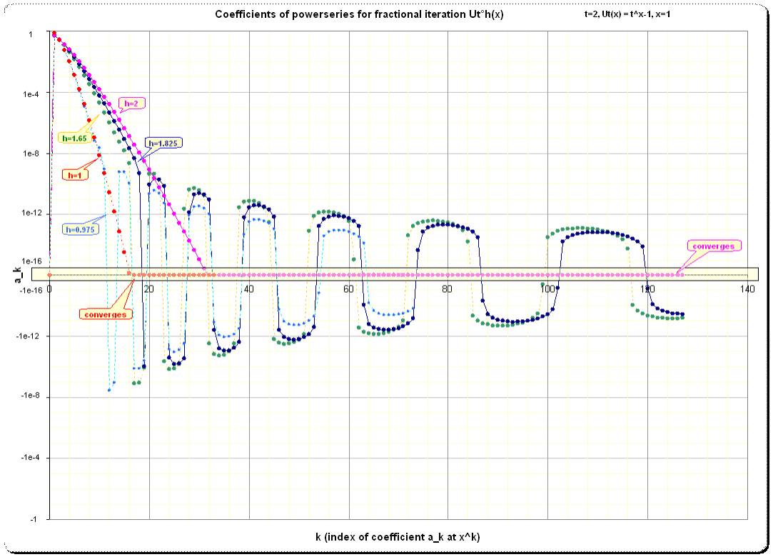
But for noninteger heights, for instance h=0.975, 1.65, 1.875 the sequences of coefficients eventually diverge. To get an idea about the characteristics of that convergent/divergent behave of the coefficients I show trajectories of a_k, k=1..128 for some example heights h (integer and fractional) and also for three different bases t.

In [Helms07-12] I show the coefficients for fractional iterates of the function U(x)=exp(x)-1, thus t=exp(1), u=1. The characteristics may be slightly different from the here-discussed series, since with t=exp(1) I used the matrix-logarithm for fractional powers and for other t I use diagonalization. The general overview over the tables of coefficients suggest, that the trajectory of absolute values of a_k starts descending to a global minimum at a certain index k, from where it continuously increases with more-than-geometric rate. The interesting impression is, that the index k disappears linearly with the logarithm of d (in h=1 + d, where d<1/2) to infinity.

Example table

            d = 1e-4           k_min=19
                 …                k_min=19
            d = 1e-10         k_min=19
            d = 1e-15         k_min=23
            d = 1e-20         k_min=25
            d = 1e-25         k_min=29
                ...                 ...

The move seems indeed to be linear in k with log(d), thus the infinite radius of convergence of the h=1 iterate is due to the fact, that d->10^-oo and the index k of the global minimum accordingly moves away to the infinity.

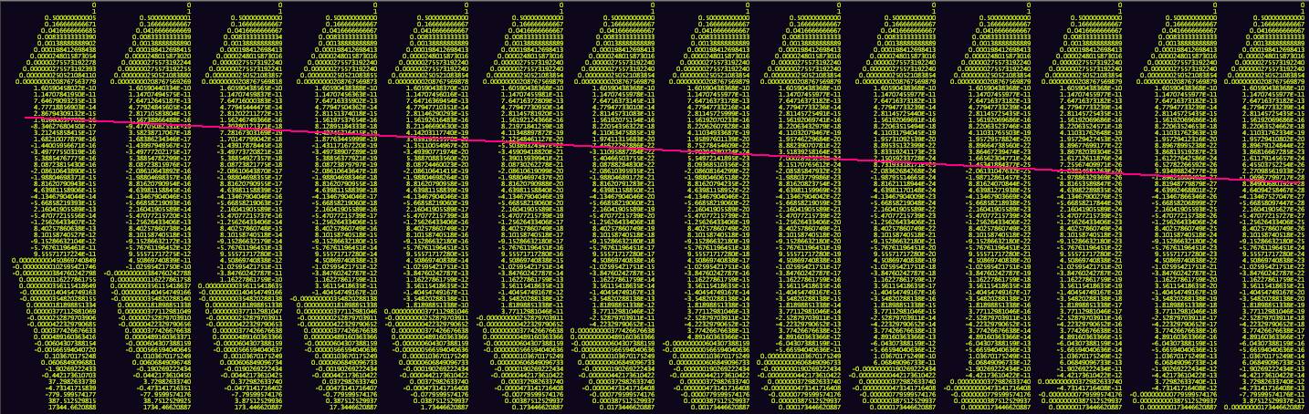
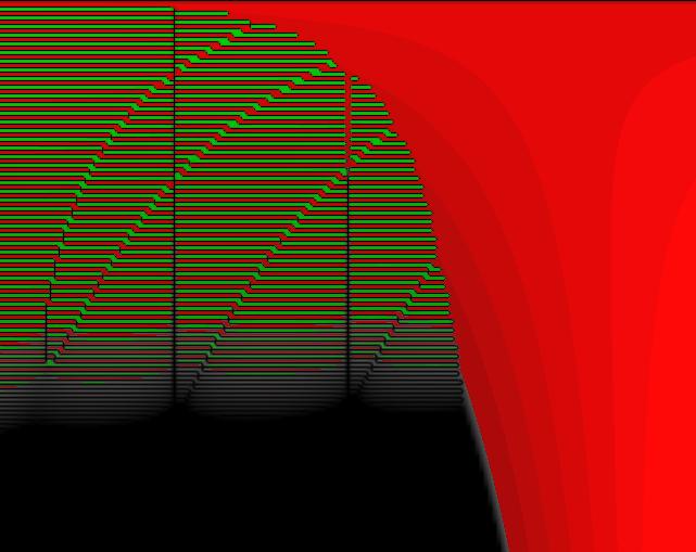
Here is a zoomed image for the coefficients of powerseries for d=10^-11, 10^-12,10^-13 ,… 10^-25 containing the ak in columns. The roughly smallest absolute values a_k (the global minima for each height) are marked by the red line

Coefficients of powerseries for different heights. The first 64 terms of each powerseries are displayed in one column

1+10-11                                                                                              1+10-15                                                                                                               1+10-20                                                                                            1+10-24	= height

 

 

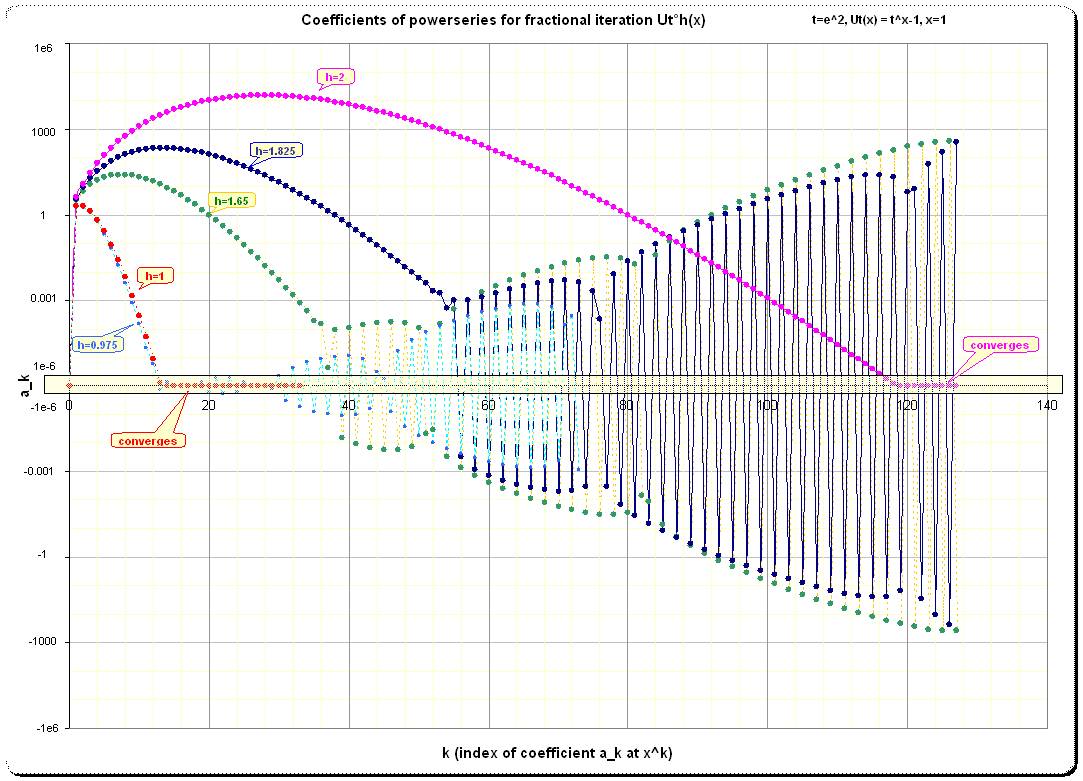
In the following plot I display the coefficents for the powerseries using t=exp(2)

I computed 128 coefficients for all example heights h.

We see the convergence of the sequence of coefficients for integer h whose graphs soon converge to the x-axis, while the a_k-sequences for fractional h have a smooth graph at the beginning but are eventually oscillating in sign and are also diverging in absolute values. Note that the y-scale is exponential.

Graph 1

 

 

In the above type of plot we cannot compare more than some example heights. To have the growthcharacteristics in a greater and more continuous overview, I show another type of plot. Here I use 161 powerseries for heights in the interval h=0..2 in equal steps.

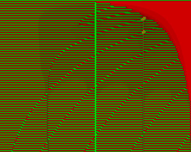
However, this mass of coefficients is difficult to print and to evaluate, if given in numbers. So here is a bitmap, whose vertical direction indicates the coefficients a_k of one powerseries (for one specific height parameter h) and the subsequent heights are the subsequent columns of one pixel for each height h. Thus the vertical column of one pixel at left border represent the coefficients of the powerseries for height h=0, the vertical line in the middle of the graph represents the coefficients of the powerseries for h=1 and the right border represents the powerseries for height h=2.

Positive coefficients are marked red and negative coefficients are marked green, with brightness-value by b_k = log(abs(a_k))/log(10), with clipping at b_k=min(max(b_k,-16),16)+sign(a_k)*16; so the brightness of the color red/green resembles roughly the index of the most significant digit of the interval 1e-16<abs(a_k)<1e16 (brightness 0<=b_k<=32)

Plot 1: Coefficients A of powerseries of different heights h 0<=h<=2

 

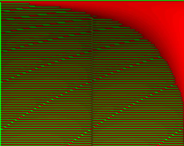
In the middle there is the vertical line for the converging-to-zero coefficients of the powerseries at h=1, and at the right border a vertical line at h=2.

In the darker area the absolute values of coefficients are smaller, in the lighter areas greater. We see an increasing of light to the bottom which indicates growth of the coefficients.

There is some more fine-structure visible: the antidiagonal lines are very obvious, but there are some brightness-areas with a very fine topology (difficult to discern in this bitmap)

 

"Pixelizing" gives a better view into the general structure:

Plot 2:

This image emphasizes some general periodicity for heights h (modulo 1).

 

In the following picture the range for h is increased. We have 0<=h<=4. The vertical lines of convergent sequences at integer h=0,1,2 are easily recognizable. The integer heights at h=3,4 do not occur as lines; the surrounding oscillations obviously occur at terms with higher index k>127.

Plot 3:

 

But we can recognize another topology of brightness now in the left bottom square. See the enhancement of this structure in the next picture.

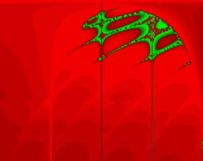
In the following picture the brightness-parameter for each pixel was logarithmized (base 10), and then a "relief "-filter was applied to the picture which renders somehow "terasses" according to the brightness-values. Here darker color of the terasses correlate with higher absolute values in the originial data and on the green line the coefficients tend to zero.

Plot 4:

 

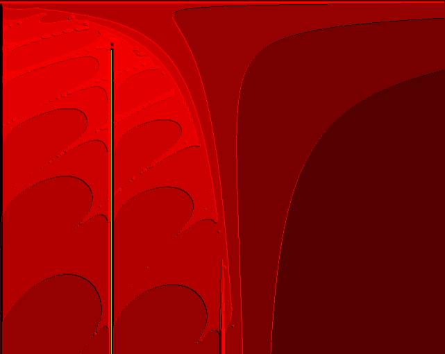
Heights –2<=h<=2

Here the original coloring scheme is used again. For higher negative h's the oscillating and diverging structure of coefficients continue and even seem to improve. The light green line is the zero-coefficients-series for h=0. (Unfortunately the program read the zeros not correctly, so assigned maximal negative values to them- the color of this line should be black, sorry.)

Plot 5: Coefficients A of powerseries

 

Accidentally I applied a "fun"-coloring-scheme – but the result is artistically impressive. It looks like the "hellgate of tetration-powerseries" – an extremely good metaphor! (Don't get lost in the chaos of that powerseries - you're now warned ...)

Plot 6: "The hellgate of tetration-powerseries"

 

 

 

Here we get wildly diverging entries, where we even don't find the larger oscillating structure of the diverging entries at fractional heights.

Since the a_k are computed by a formula, such that in the denominators occur products of

            (u-1)(u²-1)(u³-1)...(u^k-1)

where u=log(t), (see [Helms08-1],pg 21) and is here about 1.098, we have denominators near zero, which lets us expect hyperbolic effects. Indeed I could not find a larger oscillating structure is I got this in the example (using t=exp(2)) in the first 128 terms.

Graph 2:

 

 

The detail at small indexes k looks as follows

Graph 3:

 

 

 

Using base t=2 we seem to get convergent sequences of a_k.so the fractionally iterated functions U₂^oh(x) have convergence-radius of at least 1. However, for fractional iterates the sequences of coefficients have still an interesting larger-scale oscillating behaviour.

Graph 4:

 

The problem with these powerseries is that although the sequences of coefficients converge to zero and thus have a radius of convergence of at least 1, the functions of fractional heights are not well summable (Cesaro- and/or Eulersummation) and convergence cannot much be accelerated by these methods, if at all.

 

 

I possibly got an extremely simple solution for the problem of alternating divergence for fractional iteration.

We can transform the coefficients a_k of a powerseries for a fractional or integer iterate of U_t^oh(x) in the following way.

Assume the direct computation. In matrix-notation we would collect all a_k in a column-vector A and then evaluate U_t^oh(x) by the dot-product

(1)       V(x)~ * A = U_t^oh(x)

(see matrix-definitions at appendix 4.1). But we may insert a transformation by the factorially-scaled Stirling-matrix 2^nd kind U. This matrix is the operator for transforming V(x)->V(e^x -1) using base exp(1):

            V(x)~ * U = V(e^x- 1)~

 

Obviously, if we use x' = log(1+x) we have

            V(x')~ * U = V(x)~

 

So we may rewrite (1) as

            (V(x')~ * U ) * A = U_t^oh(x)

and use associativity to change order of evaluation

            V(x')~ * (U * A) = U_t^oh(x)
            V(x')~ *     A'    = U_t^oh(x)

 

We may call the expression in the parenthese A' , which is now a sort of "Stirling-transform" of A, and we observe, that the coefficients in A' form an ordinary convergent sequence.

We have then

a'k	=		where S2k,j is the Stirlingnumber 2nd kind of row k, column j of the lower triangular Stirling-matrix
Utoh(x)	=
	=

(I checked this only for the base t=exp(2) so far)

 

3.2.1.           Plot

Here is the graph of the sequences of coefficients for some fractional heights (Sorry, I used my Pari/GP-notation fS2F for U here)

Graph 5:

 

 

The graph suggests, that for all heights h>-2 (as far as tested), including the fractional ones, the sequences of coefficients converge nicely.

This transformation has another benefit: since x' = log(1+x) which is smaller than x this extends remarkably the range for the x-parameter. Possibly we have now functions, which converge for any real x.

 

 

3.2.2.           Comparision of the explicite powerseries

 

To see this explicitely written as powerseries:

The raw computation of the powerseries-expansion for U_t^o0.5(x) is:

 

U_t^o0.5(x) = 1.4142*x + 0.58579*x^2 + 0.085506*x^3 + 0.0043325*x^4 + 0.00052932*x^5 - 0.00034288*x^6
+ ...
+ 0.000054370*x^33 - 0.000035807*x^34 + 0.000010332*x^35 + 0.000022808*x^36 - 0.000064328*x^37 + 0.00011487*x^38
+...
+ 0.33002*x^87 - 0.23926*x^88 + 0.093113*x^89 + 0.12710*x^90 - 0.44514*x^91 + 0.89110*x^92 - 1.5028*x^93 + 2.3278*x^94 - 3.4251*x^95 + 4.8684*x^96 - 6.7486*x^97 + 9.1779*x^98 - 12.294*x^99 + 16.266*x^100 - 21.300*x^101 + 27.647*x^102 - 35.611*x^103 + 45.558*x^104 - 57.932*x^105 + 73.264*x^106 - 92.190*x^107 + 115.47*x^108 - 144.00*x^109 + 178.84*x^110 - 221.26*x^111 + 272.73*x^112 - 334.95*x^113 + 409.94*x^114 - 499.98*x^115 + 607.73*x^116 - 736.19*x^117 + 888.75*x^118 - 1069.2*x^119 + 1281.7*x^120 - 1530.7*x^121 + 1821.2*x^122 - 2158.0*x^123 + 2546.2*x^124 - 2990.3*x^125 + 3494.4*x^126 - 4061.1*x^127 + O(x^128)

 

which shows divergence of the coefficients, which will increase to a hypergeometric rate. The smallest coefficient occurs at x^35 (red marked) thus limits in principle the achievable accuracy.

The Stirling-transformed series for U_t', which means we have also to insert x'=log(1+x) for x, looks like

 

U_t' ^o0.5(x) = 1.4142*x + 1.2929*x^2 + 0.90699*x^3 + 0.53323*x^4 + 0.27431*x^5 + 0.12690*x^6 + 0.053781*x^7 + 0.021155*x^8 + 0.0078010*x^9 + 0.0027175*x^10 + 0.00089981*x^11 + 0.00028462*x^12 + 0.000086358*x^13 + 0.000025224*x^14 + 0.0000071125*x^15
+...
+ 1.3418e-15*x^33 - 1.8094e-16*x^34 - 2.1937e-16*x^35 + 3.0532e-16*x^36 - 2.7140e-16*x^37 + 2.0632e-16*x^38
+...
+4.9450e-28*x^87 - 9.3801e-29*x^88 - 6.8606e-29*x^89 + 1.1767e-28*x^90 - 1.1725e-28*x^91 + 9.8682e-29*x^92 - 7.6343e-29*x^93 + 5.6126e-29*x^94 - 3.9868e-29*x^95 + 2.7622e-29*x^96 - 1.8778e-29*x^97 + 1.2574e-29*x^98 - 8.3165e-30*x^99 + 5.4443e-30*x^100 - 3.5328e-30*x^101 + 2.2749e-30*x^102 - 1.4550e-30*x^103 + 9.2502e-31*x^104 - 5.8486e-31*x^105 + 3.6794e-31*x^106 - 2.3041e-31*x^107 + 1.4366e-31*x^108 - 8.9205e-32*x^109 + 5.5178e-32*x^110 - 3.4004e-32*x^111 + 2.0880e-32*x^112 - 1.2776e-32*x^113 + 7.7910e-33*x^114 - 4.7348e-33*x^115 + 2.8676e-33*x^116 - 1.7308e-33*x^117 + 1.0411e-33*x^118 - 6.2394e-34*x^119 + 3.7257e-34*x^120 - 2.2162e-34*x^121 + 1.3129e-34*x^122 - 7.7448e-35*x^123 + 4.5475e-35*x^124 - 2.6568e-35*x^125 + 1.5437e-35*x^126 - 8.9147e-36*x^127 + O(x^128)

 

with nicely diminuishing coefficients from the beginning (and even alternating).

Using x=1, while U_t^o0.5(x) has to be evaluated by means of a divergent summation technique, we get the same result by ordinary sum of the powerseries for U_t' ^o0.5 using x'=log(1+x)~0.69315 which even allows to neglect all terms from, say k=35, and we will still get a result accurate to an error smaller than something like 1e-50.

 

 

3.2.3.           Plot

 

The bitmap for 161 fractional iterates between –2<h<2 shows that nice behave in a greater overview. Here the dark area at the bottom indicates coefficients tending to zero.

Plot 7: Coefficients A' of powerseries Stirling-transformed of order 1; base t=exp(2)

 

This bitmap suggests very strongly, that indeed we can expect convergent sequences of coefficients in the powerseries for fractional iterates.

Since the powerseries for this base are "more diverging" I tried powers of U.

3.3.1.           First power of U

Bitmap by the simple Stirling-transform using U as before

Plot 8: Coefficients A' of powerseries Stirling-transformed of order 1 , base t=exp(3)

 

The transformation works as expected.

 

3.3.2.           Using second power, U²

The matrix-formula was:

(2)       V(x)~ * A = U_t^oh(x)      //restated

Using the second power of U we have to start with:

            V(x)~ * U² = V(exp(e^x- 1)-1)~

 

Now, if we use x" = log(1+log(1+x)) we have

            V(x")~ * U² = V(x)~

 

So we may rewrite (2) as

            (V(x")~ * U² ) * A = U_t^oh(x)

and use associativity to change order of evaluation

            V(x")~ * (U² * A) = U_t^oh(x)
            V(x")~ *     A"    = U_t^oh(x)

We can adapt the formula in serial notation accordingly.

 

We get the following bitmap:

Plot 9: Coefficients A" of powerseries Stirling-transformed of order 2 , base t=exp(3)

 

3.3.3.           Using third power, U³

The matrix-formula was:

(3)       V(x)~ * A = U_t^oh(x)      //restated

Using the third power of U we have to start with:

            V(x)~ * U³ = V(exp(exp(e^x- 1)-1)-1)~

 

Now, if we use x'" = log(1+log(1+log(1+x))) we have

            V(x'")~ * U³ = V(x)~

 

So we may rewrite (3) as

            (V(x'")~ * U³ ) * A = U_t^oh(x)

and use associativity to change order of evaluation

            V(x'")~ * (U³ * A) = U_t^oh(x)
            V(x'")~ *     A'"    = U_t^oh(x)

We can adapt the formula in serial notation accordingly.

 

We get the following bitmap:

Plot 10: Coefficients A'" of powerseries Stirling-transformed of order 3 , base t=exp(3)

 

Although now no black areas occur (the coefficients do not converge fast enough to zero), we can observe, that the darkening of the area read from left expands faster than the occurence of alternating signs. That may suggest, that we will asymptotically still get convergent series of coefficients, which means with convergence-radius of the function of at least 1.

 

 

3.3.4.           Hypothese

Analoguously to the classical Euler-transform in other cases of evaluating alternating divergent series, we can apply higher "orders" of the transformation. What we see is (and what are the hypotheses so far) with higher orders:

            a) the increasing size of the structures

            b) that the alternating signs disappear to the left

Here is a table of results, which is based on a slightly different implementation of this "Stirling-transformation". I use the conventional path via partial sums

           

first; setting x=1. These partial sums are then "Stirling-transformed" (with norming)

Let, for a row r denote the rowsum of U as S_r

           

(where again, S2_r,c are the Stirlingnumbers 2^nd kind) then the transforms of the partial sums are

           

and this gives then in the limit

           

In matrix-notation this is

            PS = DR * A                // where DR is the triangular unit-matrix
                                               // which implements partial summing
            U_t^oh(x) = lim _r->inf rownorm(U)*PS [r]         
                                               // where r indicates the row-index and rownorm norms
                                               //a row, such that the rowsum equals 1

The advantage of the transformation is, as said above, that we get convergent series, and – for the tested example – high accuracy with 128 terms.

 

What I got by this, using base t=exp(2) is the following table for heights –2<=h<=2 (see full table at appendix)

 

h	Utoh(1) ,128 terms used	difference of results using 128 and 127 terms	Integer iterates, direct computation
-2.000	0.148781642394	4.09201648025E-61	0.148781642394
-1.975	0.151764471472	-1.00757696730E-55
-1.950	0.154814688293	-2.20253988524E-55
-1.925	0.157934114668	-3.53513519222E-55
-1.900	0.161124633560	-4.95458163457E-55
-1.875	0.164388191607	-6.41053955877E-55
-1.850	0.167726801784	-7.85448279957E-55
...	...	...
-1.025	0.338740003829	4.52893426113E-56
-1.000	0.346573590280	5.53348935396E-123	0.346573590280
-0.9750	0.354630797379	-5.13722405573E-56
...	...
0.4500	1.91924350162	-1.75550341076E-55
0.4750	2.00205867213	-1.60763823499E-55
0.5000	2.09017531971	-1.44447235835E-55
0.5250	2.18405909158	-1.27032035841E-55
0.5500	2.28422767154	-1.08958493793E-55
...	...	...
0.9500	5.54223517697	1.54985526435E-56
0.9750	5.94359516189	8.24955710752E-57
1.000	6.38905609893	2.42197375312E-67	6.38905609893
1.025	6.88513866689	-8.97563144073E-57
1.050	7.43957118855	-1.83978085590E-56
...	...	...
1.450	45.4551347734	2.78647933160E-34
1.475	53.8234128366	1.14244842556E-32
1.500	64.3887770782	4.49621086353E-31
1.525	77.8950259312	1.70109100327E-29
1.550	95.3950973612	6.19568773605E-28
...	...	...
1.950	65150.4833093	0.0000850527607210
1.975	145391.211783	0.00190956027798
2.000	354374.278789	0.0419734968018	354374.440984

From the matrix-based formulae the effect can nicely be seen.

Since, by the matrix-approach,

            V(x)~ U_t^h = V(U_t°^h(x))~

we have by this transformation, which I expand here to a full similarity-transformation:

            (V(log(1+x))~ *U )* U_t^h  = V(U_t°^h(x))~
            (V(log(1+x))~ *(U * U_t^h *U^-1 )            = V(U_t°^h(x))~ *U^-1
                                                                       =  V(log(1+U_t°^h(x)))~
            U * U_t^h *U^-1     =  U * (^dV(u) U)^h *U^-1
                                   = (^dV(1/u) ^dV(u))* U * (^dV(u) U)^h-1 * ^dV(u) U*U^-1
                                   =  ^dV(1/u) (^dV(u)* U * (^dV(u) U)^h-1 )* ^dV(u) 
                                   =  ^dV(1/u) (^dV(u) U)^h* ^dV(u) 
(1)                              =  ^dV(1/u) *  U_t^h * ^dV(u) 

which also results in the transformation

            V(log(1+x)/u)~ * U_t^h  = V(log(1+U_t°^h(x))/u)~

The effect of (1) is, that in the symbolic powerseries we remove just powers of u. Recall the the symbolic powerseries for U_t°^h(x):

            U_t°^h(x) =

where a_u,k(u^h) are polynomials in u and u^h with coeffients depending on k, we have also the factor u_k. This u_k- factor disappears by the similarity-transformation in the following way

            U_t°^h(x) =

But since this is only the removal of a factor with geometric increase, but the powerseries seem to have convergence-radius zero (hypothetically extending I.N.Baker's result for exp(x)-1), we are not yet definitely on the succes-side. However, since many more terms of the powerseries are decreasing in absolute value, we should be able to get better approximations this way, at least for bases t, where u=log(t)>1 .

 

(to be continued)

The difficult to handle powerseries for fractional iteration seem to be transformable into convergent series by a simple transform using the Stirlingnumbers 2^nd kind.

 

Gottfried Helms, 24.07.2008

 

All derivations are done in the matrix-notation; however can be re-expressed in common serial notation. The matrix-notation is simply meant to keep the formulae concise.

All matrices are assumed as of infinite size (to resemble the infinite terms of powerseries); in the current computations I truncated them to size n=128 resp nxn=128x128.

The used matrix-operators for the U-tetration are named U resp. U_t and the other involved standard-matrices are as follows:

            V(x)     :=  column_r=0..inf[1,x,x²,x³,...x^r,...]
                        an infinite "vandermonde" (column-) vector of a general x
            V(x)~   := the transpose ; the symbol is taken from the convention in Pari/GP
            ^dV(x)    := the diagonal arrangement of V(x)
           

            The column- and rowindices are beginning at zero

VZ          := matrixr=0..inf,c=0..inf[cr]                := [V(0),V(1),V(2),...]                the collection of V()-vectors of consecutive parameters
P            := matrixr=0..inf,c=0..inf[binomial(r,c)]                 the lower-triangular Pascal-matrix
dF           := diag(0!,1!,2!,...)
S2           :=  matrixr=0..inf,c=0..inf[s2r,c]                // s2 Stirling-numbers 2nd kind
S1           :=  matrixr=0..inf,c=0..inf[s1r,c]                      // s1 Stirling-numbers 1st kind
U = fS2F:=  matrixr=0..inf,c=0..inf[s2r,c c!/r!]                // s2 Stirling-numbers 2nd kind
u            :=log(t)                       // base-parameter Ut           := dV(u) * U
DR          := matrixr=0..inf,c=0..inf[if(r>=c,1)]

 

The function U_t°^h(x) can be computed by the dot-product of V(x) and column 1 of the h^th-power of U_t (which contains the required coefficients of the powerseries)

            V(x)~ * U_t^h      = V(U_t°^h(x) )~

or, referencing the second column of U_t only:

            V(x)~ * U_t^h [,1]            = U_t°^h(x)

The fractional powers of the matrix U_t is computed by diagonalization:

            U_t = W^-1 * D * W         // where the diagonal D equals ^dV(u) and W is triangular

This can exactly be solved for any finite dimension where the entries are constant wrt to selected matrix-size. (A simple recursive solution). Then the fractional h'th powers of U_t are computed by

            U_t^h = W^-1 * ^dV(u^h) * W           

Important: for u=1, t=exp(1) (and bases near that value) the matrix-logarithm is applied instead.

 

4.2.1.           Base t=exp(2)

 

Table of approximates of U_t^oh(1) for h=-2..2 in 160 steps using base t=exp(2)~6.38905609893

h	Utoh(1) 128 terms used	difference of results using 128 and 127 terms
-2.000	0.148781642394	4.09201648025E-61
-1.975	0.151764471472	-1.00757696730E-55
-1.950	0.154814688293	-2.20253988524E-55
-1.925	0.157934114668	-3.53513519222E-55
-1.900	0.161124633560	-4.95458163457E-55
-1.875	0.164388191607	-6.41053955877E-55
-1.850	0.167726801784	-7.85448279957E-55
-1.825	0.171142546188	-9.24093772260E-55
-1.800	0.174637578968	-1.05285638946E-54
-1.775	0.178214129401	-1.16810569215E-54
-1.750	0.181874505127	-1.26678601269E-54
-1.725	0.185621095548	-1.34646777765E-54
-1.700	0.189456375403	-1.40537883466E-54
-1.675	0.193382908532	-1.44241617525E-54
-1.650	0.197403351836	-1.45713893941E-54
-1.625	0.201520459451	-1.44974402527E-54
-1.600	0.205737087133	-1.42102600088E-54
-1.575	0.210056196899	-1.37232332072E-54
-1.550	0.214480861902	-1.30545308365E-54
-1.525	0.219014271584	-1.22263673030E-54
-1.500	0.223659737106	-1.12641916825E-54
-1.475	0.228420697091	-1.01958383306E-54
-1.450	0.233300723675	-9.05066148888E-55
-1.425	0.238303528916	-7.85867746245E-55
-1.400	0.243432971557	-6.64973635962E-55
-1.375	0.248693064184	-5.45274331996E-55
-1.350	0.254087980802	-4.29494671718E-55
-1.325	0.259622064847	-3.20130807787E-55
-1.300	0.265299837682	-2.19396550105E-55
-1.275	0.271126007591	-1.29179928123E-55
-1.250	0.277105479321	-5.10105315764E-56
-1.225	0.283243364195	1.39621203423E-56
-1.200	0.289544990856	6.49792278030E-56
-1.175	0.296015916665	1.01672701607E-55
-1.150	0.302661939812	1.24055075057E-55
-1.125	0.309489112197	1.32500139054E-55
-1.100	0.316503753120	1.27715294403E-55
-1.075	0.323712463854	1.10706770668E-55
-1.050	0.331122143163	8.27389786305E-56
-1.025	0.338740003829	4.52893426113E-56
-1.000	0.346573590280	5.53348935396E-123
-0.9750	0.354630797379	-5.13722405573E-56
-0.9500	0.362919890491	-1.07006321730E-55
-0.9250	0.371449526905	-1.65066443311E-55
-0.9000	0.380228778734	-2.23749445643E-55
-0.8750	0.389267157395	-2.81328981940E-55
-0.8500	0.398574639809	-3.36195528409E-55
-0.8250	0.408161696458	-3.86891434953E-55
-0.8000	0.418039321439	-4.32140384738E-55
-0.7750	0.428219064697	-4.70870803363E-55
-0.7500	0.438713066612	-5.02232933208E-55
-0.7250	0.449534095129	-5.25609461431E-55
-0.7000	0.460695585670	-5.40619756770E-55
-0.6750	0.472211684045	-5.47117927292E-55
-0.6500	0.484097292638	-5.45185054828E-55
-0.6250	0.496368120150	-5.35116089595E-55
-0.6000	0.509040735221	-5.17401997699E-55
-0.5750	0.522132624272	-4.92707843411E-55
-0.5500	0.535662253964	-4.61847555857E-55
-0.5250	0.549649138683	-4.25756175589E-55
-0.5000	0.564113913536	-3.85460400264E-55
-0.4750	0.579078413362	-3.42048250880E-55
-0.4500	0.594565758348	-2.96638661656E-55
-0.4250	0.610600446866	-2.50351759218E-55
-0.4000	0.627208456258	-2.04280541998E-55
-0.3750	0.644417352338	-1.59464601053E-55
-0.3500	0.662256408490	-1.16866441150E-55
-0.3250	0.680756735328	-7.73508687414E-56
-0.3000	0.699951422006	-4.16678141471E-56
-0.2750	0.719875690386	-1.04388516000E-56
-0.2500	0.740567063404	1.58524242474E-56
-0.2250	0.762065549163	3.68661106455E-56
-0.2000	0.784413842431	5.24078433084E-56
-0.1750	0.807657545455	6.24269166760E-56
-0.1500	0.831845410221	6.70109033021E-56
-0.1250	0.857029604574	6.63770739168E-56
-0.1000	0.883266004898	6.08609846115E-56
-0.07500	0.910614518426	5.09026502228E-56
-0.0500	0.939139438629	3.70307626659E-56
-0.0250	0.968909837620	1.98454393587E-56
0.0000	1.00000000000	2.041281526E-202
0.0250	1.03248990321	-2.18177298377E-56
0.0500	1.06646575014	-4.49041019351E-56
0.0750	1.10202056051	-6.85578525869E-56
0.1000	1.13925482862	-9.20974045399E-56
0.1250	1.17827725587	-1.14876877214E-55
0.1500	1.21920556807	-1.36300468824E-55
0.1750	1.26216742863	-1.55834930026E-55
0.2000	1.30730146082	-1.73019908921E-55
0.2250	1.35475839393	-1.87476010084E-55
0.2500	1.40470235077	-1.98910473981E-55
0.2750	1.45731229648	-2.07120446227E-55
0.3000	1.51278367212	-2.11993867020E-55
0.3250	1.57133023995	-2.13508068412E-55
0.3500	1.63318617222	-2.11726219652E-55
0.3750	1.69860842041	-2.06791807521E-55
0.4000	1.76787940830	-1.98921378529E-55
0.4250	1.84131009978	-1.88395802419E-55
0.4500	1.91924350162	-1.75550341076E-55
0.4750	2.00205867213	-1.60763823499E-55
0.5000	2.09017531971	-1.44447235835E-55
0.5250	2.18405909158	-1.27032035841E-55
0.5500	2.28422767154	-1.08958493793E-55
0.5750	2.39125782952	-9.06643473920E-56
0.6000	2.50579359389	-7.25740373036E-56
0.6250	2.62855575211	-5.50887633339E-56
0.6500	2.76035292858	-3.85775699610E-56
0.6750	2.90209454058	-2.33696348512E-56
0.7000	3.05480599903	-9.74789623601E-57
0.7250	3.21964660129	2.05588436331E-57
0.7500	3.39793066465	1.18645675450E-56
0.7750	3.59115257551	1.95575725626E-56
0.8000	3.80101658899	2.50713260877E-56
0.8250	4.02947241486	2.83982801087E-56
0.8500	4.27875788211	2.95845886162E-56
0.8750	4.55145030117	2.87265617216E-56
0.9000	4.85052856291	2.59660405743E-56
0.9250	5.17944855466	2.14848564740E-56
0.9500	5.54223517697	1.54985526435E-56
0.9750	5.94359516189	8.24955710752E-57
1.000	6.38905609893	2.42197375312E-67
1.025	6.88513866689	-8.97563144073E-57
1.050	7.43957118855	-1.83978085590E-56
1.075	8.06155846276	-2.79887303842E-56
1.100	8.76212065682	-3.74458219387E-56
1.125	9.55452324610	-4.34775784184E-56
1.150	10.4548261171	2.06904925500E-55
1.175	11.4825897977	2.03275257844E-53
1.200	12.6617904993	1.48421551843E-51
1.225	14.0220149408	1.01379756997E-49
1.250	15.6000333024	6.51488362789E-48
1.275	17.4418878886	3.94903550037E-46
1.300	19.6056919163	2.26333836768E-44
1.325	22.1654160710	1.22932849531E-42
1.350	25.2160637847	6.34129229359E-41
1.375	28.8808211306	3.11286011567E-39
1.400	33.3210482169	1.45695775320E-37
1.425	38.7504117507	6.51372560175E-36
1.450	45.4551347734	2.78647933160E-34
1.475	53.8234128366	1.14244842556E-32
1.500	64.3887770782	4.49621086353E-31
1.525	77.8950259312	1.70109100327E-29
1.550	95.3950973612	6.19568773605E-28
1.575	118.404353175	2.17527216428E-26
1.600	149.142852032	7.37145701535E-25
1.625	190.926311527	2.41399561943E-23
1.650	248.811306070	7.64832842296E-22
1.675	330.686113737	2.34705994831E-20
1.700	449.164016764	6.98342783166E-19
1.725	624.964213535	2.01668882457E-17
1.750	893.139076207	5.65789354699E-16
1.775	1314.93820096	1.54354082962E-14
1.800	2001.26271589	4.09839428311E-13
1.825	3160.95197578	1.06001083639E-11
1.850	5204.73282794	0.000000000267276805071
1.875	8980.30615555	0.00000000657514974489
1.900	16333.8660823	0.000000157931503896
1.925	31535.3809448	0.00000370649148228
1.950	65150.4833093	0.0000850527607210
1.975	145391.211783	0.00190956027798
2.000	354374.278789	0.0419734968018

 

 

[Bak]                      Baker, Irvine Noel;
Zusammensetzungen ganzer Funktionen
1958; Mathematische Zeitschrift, Vol 69, Pg 121-163,

[Vol]                      Volkov, I.I.;
Riesz summation method
Online reference Springer:Encyclopaedia of Mathematics
Edited by Michiel Hazewinkel
online at http://eom.springer.de/r/r082300.htm

[Helms,07-11]     Helms, Gottfried;
Coefficients for fractional iterations of the U-function (first version)
online at http://go.helms-net.de/math/tetdocs/CoefficientsForUTetration.htm

[Helms,07-12]     Helms, Gottfried;
Coefficients for fractional iterations of the U-function (extended version)
online at http://go.helms-net.de/math/tetdocs/htmltable_utetrationFractionalIteration.htm

[Helms,08-1]       Helms, Gottfried;
Continuous functional iteration
pg 21, online at http://go.helms-net.de/math/tetdocs/ContinuousfunctionalIteration.pdf